OPULENT VOICE AND HAIFURAIYA, AN OPEN-SOURCE TECHNICAL BASELINE FOR THE NEXT GEOSTATIONARY AMATEUR RADIO PAYLOAD
A white paper for presentation at the futureGEO Community Workshop HAM RADIO 2026, Friedrichshafen Saturday, 27 June 2026 Hosted by AMSAT-DL e.V. with the ESA Satellite Communications Group
Author: Michelle Thompson W5NYV on behalf of ORI A 501(c)(3) all-volunteer open-source nonprofit https://www.openresearch.institute
Version 1.0 — May 2026
1. EXECUTIVE SUMMARY
The amateur radio satellite community is asked, at HAM RADIO 2026, what should come after Qatar-OSCAR 100. AMSAT-DL and the ESA Satellite Communications Group have framed three concepts for discussion: an evolutionary bent-pipe successor (Enhanced QO-100+), a software-defined regenerative payload (Digital Innovation Lab), and an exploratory mm-wave pathfinder.
The Open Research Institute proposes that a regenerative, software-defined path is the best way forward. None of the concepts are a perfect alignment, but Concept 2 is the closest fit. The next step with regenerative software-defined hardware is the best next step, and that step can be taken now, with substantially reduced risk, because the necessary open-source building blocks exist and have been and are being demonstrated.
This paper describes those building blocks. It describes the Opulent Voice (OPV) air interface and the Haifuraiya (“High Flyer”) system architecture that uses it. It describes the working demonstration hardware that ORI is bringing to the workshop: a complete FDMA uplink modem, a C++ reference modulator and demodulator, a human-radio user interface, the Pluto-side ARM application stack, and a hardware-verified DVB-S2 transmit chain suitable for the downlink. It explains why open-licensing this stack serves amateur radio better than any alternative on offer.
The claim made here is firm: an open, regenerative, voice-and- data unified architecture, built on the demonstrated Opulent Voice / Haifuraiya stack, best serves the international amateur radio community in geostationary orbit.
2. WHAT QO-100 TAUGHT US
QO-100, Es’hail-2’s narrowband and wideband amateur transponders, has been an extraordinary success. It proved that geostationary amateur access is technically and operationally viable, that a bent-pipe transponder remains a workhorse, and that even a modest amateur payload, well placed, can transform the daily life of thousands of operators.
QO-100 also taught us where the limits lie:
A bent-pipe transponder cannot perform onboard processing. Spectrum is shared, not allocated. Misbehavior on the uplink lands directly on the downlink. There is no system discipline beyond operator etiquette.
Modulation and access are constrained by what each operator can transmit. The transponder cannot impose framing, FEC, or scheduling.
Bandwidth is finite, and so is downlink EIRP. Many users share a fixed pipe. Quality degrades with offered load.
Voice quality, when digital voice is used at all, depends on legacy low-bitrate codecs designed for narrowband VHF repeaters. Codec 2 at 3.2 kbps, AMBE at 3.4 kbps. These voice encoders deliver quality that is technically a very long way behind what mobile telephony has offered for over two decades.
Modes are siloed. Switching from voice to data, or voice to image, means stopping, retuning, and starting again on a separate scheme.
A successor payload that simply does more of the same will inherit all of these constraints. A regenerative, software-defined payload removes them.
3. THE OPULENT VOICE PROTOCOL
Opulent Voice is ORI’s open-source, patent-free digital voice and data protocol for amateur radio. The current specification is OPV Protocol v1.1 (January 2026). All parameters in this section are taken verbatim from the protocol specification and the published reference implementations.
3.1 Design Philosophy
OPV is built on five principles:
Voice always wins. Voice transmission has absolute priority over all other traffic types, with carefully bounded exceptions for authentication.
Modern codec quality. Opus is used at a minimum of 16 kbps, delivering audio quality that exceeds amateur expectations set by Codec 2 (3.2 kbps) and AMBE (3.4 kbps).
Unified protocol. One frame format carries voice, text, file transfer, control, and authentication. There is no mode switching. Priority queues and UDP port assignment handle multiplexing.
Open source. Every block of the protocol is fully documented, patent-free, and available under internationally recognized open licenses.
40 ms frame timing. The reference implementation aligns the air interface to the 40 ms Opus audio callback, so one voice packet exactly fills one over-the-air frame.
The 24-bit sync word 0x02B8DB was selected by exhaustive search of all 24-bit sequences. Of the 6,864 sequences that achieve an 8:1 peak-to-secondary-lobe ratio in the soft correlation output, 0x02B8DB is one, and it is mnemonic: “Oh to be eight dB!”
3.3 Frame Structure
The pre-encoding OPV frame is 134 bytes, structured as:
Offset
Size
Field
0 – 5
6 bytes
Station ID (Base-40 callsign encoding)
6 -8
3 bytes
Authentication token
9 – 11
3 bytes
reserved
12 – 133
122 bytes
voice, control, text, data payload
After randomization, rate-1/2 convolutional encoding, and 67×32 block interleaving, the payload occupies 2144 bits. The 24-bit sync word brings the on-air frame to 2168 symbols, or exactly 40 ms at 54,200 baud.
3.4 Higher Layers
Above the physical layer, OPV uses standard internet conventions:
IP/UDP for transport.
RTP for Opus voice payloads, de-jitter, and station ID hash.
COBS (Consistent Overhead Byte Stuffing) for framing variable-length data that may span multiple OPV frames.
Per-frame Base-40-encoded station identification.
Per-frame authentication token enabling controlled access without proprietary encryption.
This is the protocol stack used in ORI’s terrestrial point-to- point Opulent Voice demonstrations and in the Haifuraiya satellite reference design.
4. THE DEMONSTRATION HARDWARE
ORI is bringing the following working, open-source designs to the futureGEO Community Workshop. All are public repositories under github.com/OpenResearchInstitute, and all are inspectable, buildable, and modifiable today.
4.1 pluto_msk — The Uplink Modem (VHDL / FPGA)
The pluto_msk repository is an Opulent Voice MSK modem targeting the AMD Zynq Z-7020 SoC inside the Analog Devices “PLUTO clone” SDRS. The modem and supporting blocks come from ORI’s open RTL library:
msk_modulator
msk_demodulator
nco (numerically controlled oscillator)
pi_controller (proportional-integral loop)
prbs (pseudo-random bit sequence generator)
power_detector
lowpass_ema (exponential moving average filter)
The current design targets the LibreSDR platform (Zynq 7020 with LVDS interface to the AD9363 transceiver).
4.2 opv-cxx-demod — C++ Reference Modulator and Demodulator
A self-contained C++ implementation of both the OPV modulator and demodulator, designed to interoperate with the FPGA modem and with Interlocutor. It runs on a host computer alongside PlutoSDR or LibreSDR hardware. It is the reference for the air-interface, and verifies that the FPGA implementation matches the protocol specification bit-for-bit.
License: GPLv3.
4.3 dialogus — Pluto ARM/Linux Application
C-code applications that run on the ADALM-Pluto’s ARM cores inside the Zynq processing system. Dialogus is the device-side companion to Interlocutor, handling IIO operations, frame header construction, FEC, interleaving, randomization, MSK register configuration, statistics, and UDP encapsulation. It is the production-grade glue that makes the FPGA modem and the user interface work together.
License: GPLv3.
4.4 Interlocutor — Human-Radio Interface
A Python-based human-radio interface for Opulent Voice. It provides a web GUI, voice input and output, real-time text chat, slash-command extensions for operator workflow, and an audio device management layer. It is the user-facing terminal that turns the FPGA modem and the Pluto application into an actual amateur radio station. It has been deployed in full- duplex interoperability tests between PlutoSDR and LibreSDR.
License: GPLv3.
4.5 dvb_fpga — DVB-S2 Downlink Encoder
The dvb_fpga repository implements RTL components for a full DVB-S2 transmitter. All six core blocks are verified in simulation, in hardware testing, and the design is currently used for Q0-100 stations in the EU:
Per-frame parameter switching with no reset required
Behavior is validated to match GNU Radio’s DVB-S2 reference output. License: CERN-OHL-W.
This block is exactly what a Haifuraiya-style regenerative payload needs on its downlink: a re-modulator that takes multiplexed amateur traffic and emits a single, standards- compliant, ground-receivable DVB-S2/S2X signal.
4.6 What This Adds Up To
Considered together, these repositories constitute a complete, open-source, FPGA-and-software amateur radio communications system:
5. HAIFURAIYA: THE SYSTEM ARCHITECTURE
Haifuraiya, or “High Flyer”, is ORI’s reference geostationary mission concept. The architecture is described in the ORI public documentation set and summarized here from the OPV multiplexing reference document.
Many single-channel FDMA uplinks from ground-station user terminals, each one an Opulent Voice signal as described in Section 3, are received by the satellite. Each uplink is demodulated on board. Demodulated OPV frames carry, in their headers, the transmitting station’s Base-40 callsign and an authentication token. The payload determines whether the satellite forwards the frame, in accordance with the AAAAA protocol (access, authentication, authorization, accounting, auditing). Accepted frames are multiplexed onto a single DVB-S2/S2X downlink.
This is a regenerative payload. The satellite does not relay RF; it processes packets. That has significant consequences.
The uplink and downlink are decoupled. Misbehavior on one uplink does not corrupt the downlink for everyone else. The satellite can mute, rate-limit, or drop bad actors at the source.
Spectrum is used efficiently. FDMA uplinks at modest baud rate aggregate cleanly onto a wide downlink at one of the high-rate DVB-S2 modcods.
The downlink is receivable with standard, inexpensive, widely available consumer DVB-S2 hardware. Every amateur on the planet has access to receive equipment.
Per-frame authentication enables coordinated access without closing the system. Amateur openness is preserved; abuse is bounded.
The system can carry voice, text, files, telemetry, and IoT traffic in one unified protocol, exactly as concept 1 in the workshop call envisions. Except we do this natively, without bolting features on top of a bent pipe.
Haifuraiya is not a bent-pipe-plus. It is a different class of mission, and it is closest to the class of mission concept 2 of the workshop description points toward.
6. MAPPING TO THE THREE WORKSHOP CONCEPTS
The workshop call presents three concepts. ORI’s Haifuraiya proposal relates to each as follows.
Concept 1 — Enhanced QO-100+ (Evolutionary)
The Enhanced QO-100+ concept proposes “classic bent-pipe narrowband and wideband transponders, an advanced beacon architecture, multi-band downlinks and additional functions such as text and image transmission, e.g. for emergency and disaster communication, IoT.”
Every “additional function” listed is a native, designed-in capability of Opulent Voice. Voice, text, image data, control, and IoT-class telemetry share one frame format with priority queuing. Where Concept 1 must add features to a bent pipe, Haifuraiya already has them.
Concept 2 — Digital Innovation Lab (Regenerative SDR)
This is the natural home of the Haifuraiya / Opulent Voice architecture. The workshop call notes a single risk for this concept: “the risk of being very software-heavy.” Section 8 below addresses that risk directly. The short form: the heavy lifting is in FPGA RTL, not in CPU software, and the RTL is already implemented, simulated, and verified on hardware.
Concept 3 — High Frequency Pathfinder (mm-wave)
ORI does not propose Haifuraiya as a replacement for an mm-wave pathfinder. The two are complementary. An open digital baseband stack like Opulent Voice / dvb_fpga is, in fact, exactly what a pathfinder needs in its supporting telemetry, beacon, and experimental data paths.
7. WHY OPEN SOURCE BEST SERVES AMATEUR RADIO
7.1 Patent-Free, License-Friendly
The Opulent Voice voice codec is Opus, a royalty-free, patent- free standard developed by the IETF. There are no per-radio license fees, no proprietary vocoder ICs, no export-controlled algorithms, no surprise patent claims. By contrast, every commercial amateur digital voice system in widespread use today depends on proprietary, royalty-bearing vocoders that cannot be freely implemented, freely shared, or freely modified.
7.2 Inspectable and Auditable
Every block in the Haifuraiya stack, the physical layer modulation, FEC, interleaving, randomization, framing, multiplexing, downlink encoder, is published source. Any amateur, any institution, and any regulator can verify exactly what is happening on the air. Open inspection is a prerequisite for amateur radio in jurisdictions that prohibit unlicensed encryption.
7.3 Distributable and Modifiable
CERN-OHL-W (used by pluto_msk and dvb_fpga) and GPLv3 (used by Interlocutor, Dialogus, and opv-cxx-demod) are recognized open licenses with strong reciprocity. Anyone can fork, port, improve, or replace any block. Anyone, anywhere can compile the bitstream. Different SDR platforms can host the design. Standards committees can incorporate it. None of this requires asking permission from a vendor.
7.4 Educational
Open hardware and open software are the most powerful teaching tools amateur radio possesses. Students can read the VHDL, run the simulations, watch the constellation, change a parameter, and learn. A closed-source satellite payload teaches nothing beyond its user interface.
7.5 Long-Lived
Open designs outlive their original maintainers. The CERN-OHL and GPL ecosystems are demonstrably durable. A bent-pipe analog payload is, ultimately, a single point of failure. An open, regenerative payload’s reference design is preserved indefinitely, can be re-flown, and can be extended.
8. ADDRESSING THE “SOFTWARE-HEAVY” RISK
The workshop description identifies a single risk for the Digital Innovation Lab concept: “But with the risk of being very software-heavy.” This concern deserves a direct response.
8.1 The Heavy Lifting Is in FPGA, Not CPU
The OPV modem, the demodulator, the FEC, the interleaver, the multiplexer, and the downlink DVB-S2 encoder all live in FPGA fabric. They are deterministic, real-time, and timing-closed. They are not running as Python or C on a general-purpose CPU. This is not software in the sense the workshop call is worried about; it is hardware design expressed in HDL. Demodulation and decoding done in software is done with validated and verified routines in dedicated processors, such as the A53 quad core on the ZCU102.
8.2 The FPGA Designs Exist and Have Been Built
Every block named in this paper has been synthesized, place- and-routed, and run on real silicon. The pluto_msk modem has been built for both PlutoSDR (Zynq 7010) and LibreSDR (Zynq 7020 with LVDS). The dvb_fpga blocks are verified in both simulation and hardware testing. We are not asking the amateur satellite community to fund a research program. We are asking it to adopt designs that already work.
8.3 The Air Interface Has Been Flown Terrestrially
Full-duplex Opulent Voice interoperability has been demonstrated end-to-end between Interlocutor with opv-cxx-demod on PlutoSDR, and Dialogus with the FPGA modem (Locutus) on LibreSDR. The protocol works. The implementation works. What remains is space qualification, not invention.
8.4 The Operating System Layer Is Small
The Pluto-side ARM application is C, not a heavy framework. The user terminal is Python, not a stack of microservices. It was deliberately designed to be internet-free, HTML5/CSS/Javascript only, and accessible by design. The complexity budget is dominated by the deterministic FPGA path. Software is a complement, not a foundation.
9. WHAT ORI PROPOSES
ORI proposes that the futureGEO Community Workshop:
Adopt regenerative onboard processing as the technical baseline for the next amateur radio geostationary payload.
Adopt Opulent Voice as the uplink air-interface reference, in coordination with the IEEE P1954 standards effort.
Adopt DVB-S2/S2X as the downlink, using the open-source dvb_fpga implementation as the reference encoder.
Adopt the Haifuraiya FDMA-uplink / multiplexed-downlink architecture as the system reference.
Treat the demonstration hardware presented at HAM RADIO 2026 as the starting point for a working group, not as a finished product, with a written collaboration framework between participating organizations.
ORI commits, for its part, to continued open development, public availability of every block under CERN-OHL-W or GPLv3, formal written partnership agreements with collaborators, and ongoing standards-track contributions through IEEE P1954.
10. CONCLUSION
Qatar-OSCAR 100 is a landmark. The next amateur radio geostationary payload should be a landmark of a different kind: the first regenerative, fully open-source, voice-and-data unified amateur GEO mission in history. The technology to build it is on the table at HAM RADIO 2026. The licensing is permissive. The protocols are documented. The hardware works.
This is what best serves amateur radio.
APPENDIX A — OPULENT VOICE TECHNICAL PARAMETERS
Modulation MSK Symbol rate 54,200 baud Frequency deviation +/- 13,550 Hz Frame duration 40 ms Frame length 2168 symbols Sync word 0x02B8DB (24 bits) Sync PSLR 8:1 (soft correlation) Channel code Rate-1/2, K=7 convolutional G1 = 0x4F (171 octal) G2 = 0x6D (133 octal) Interleaver 67 × 32 block with bit reversal Randomizer CCSDS 8-bit LFSR x^8 + x^7 + x^5 + x^3 + 1 Payload (pre-encoding) 134 bytes Station ID 6 bytes (Base-40) Authentication token 3 bytes Reserved 3 bytes Voice / data 122 bytes Voice codec Opus, ≥ 16 kbps Transport IP / UDP, RTP for voice Framing COBS License (RTL) CERN-OHL-W License (software) GPLv3
OPULENT VOICE AND HAIFURAIYA A Working Open-Source Path for the Next GEO Amateur Radio Open Research Institute (ORI), a 501(c)(3) all-volunteer open-source nonprofit, https://www.openresearch.institute
Submitted to the futureGEO Community Workshop HAM RADIO 2026, Friedrichshafen Saturday, 27 June 2026 Michelle Thompson (W5NYV) CEO Paul Williamson (KB5MU) Remote Labs Lead
OUR POSITION
A digitally regenerative, software-defined GEO amateur radio payload is the right next step after QO-100. And, it is not a leap of faith. ORI is bringing the working open-source hardware and software that proves this path. We are demonstrating the signal chain in Friedrichshafen.
WHAT WE ARE BRINGING TO HAM RADIO 2026
pluto_msk — OPV uplink MSK modem in VHDL, running on PLUTO SDR clone hardware (AMD Zynq Z-7020). CERN-OHL-W open hardware license.
opv-cxx-demod — Full C++ Opulent Voice modulator and demodulator for PlutoSDR / LibreSDR. GPLv3.
dialogus — ARM/Linux application stack running on the Pluto’s Zynq processing system. Production-grade C code.
Interlocutor — Human-radio interface with web GUI, voice, text chat, slash-command extensions, and full operator workflow. Python. GPLv3.
dvb_fpga — DVB-S2 transmitter RTL: scrambler, BCH, LDPC, bit-interleaver, constellation mapper, physical-layer framing. All six core components verified in simulation AND in hardware. Frame types: Normal and Short. Constellations: 8PSK, 16APSK, 32APSK. Code rates 1/4 through 9/10. CERN-OHL-W.
This is the uplink, the downlink encoder, the user terminal, and the air interface. All open source, all working, all available for inspection online and in person.
OPULENT VOICE — VERIFIED PARAMETERS
Modulation MSK (Minimum Shift Keying) Symbol rate 54,200 baud Frequency dev. +/- 13,550 Hz Frame duration 40 ms (2168 symbols) Sync word 0x02B8DB (24 bits, optimized 8:1 PSLR) FEC Rate-1/2 K=7 convolutional (171/133 octal) Interleaver 67×32 block with bit reversal Randomizer CCSDS 8-bit LFSR (x^8+x^7+x^5+x^3+1) Voice codec Opus, 16 kbps minimum Transport IP/UDP/RTP, COBS framing Authentication Per-frame Base-40 station ID + token
HAIFURAIYA — THE SYSTEM ARCHITECTURE
Haifuraiya (“High Flyer”) is ORI’s reference GEO mission concept. Many single-channel FDMA Opulent Voice uplinks are received by the satellite, demodulated on board, and multiplexed onto a single DVB-S2/S2X downlink. Per-frame station identification and authentication enable controlled access without sacrificing amateur openness. The downlink encoder needed for this concept is exactly the dvb_fpga we are demonstrating. Haifuraiya is implemented with a modern and efficient polyphase filter bank and channelizer.
WHY THIS BEST SERVES AMATEUR RADIO
OPEN. CERN-OHL-W hardware and GPLv3 software. Patent-free codec (Opus). No proprietary vocoders. No low-rate vocoders. No export-controlled IP. Every amateur on the planet can build, modify, study, and improve every block.
UNIFIED. Voice, text, file, control, and IoT traffic share one frame format with priority queuing. No mode switching. The “additional functions” that Concept 1 wants to add to QO-100+ are already a native part of OPV.
MODERN VOICE QUALITY. Opus at 16 kbps decisively exceeds legacy 3.2–3.4 kbps digital voice modes (Codec 2, AMBE). Amateurs deserve to hear each other clearly.
DE-RISKED. The “software-heavy” concern raised against the Digital Innovation Lab concept is answered by FPGA RTL that has been built, simulated, and run on hardware. The heavy lifting lives in fabric, not in CPU instructions.
STANDARDS-TRACK. OPV PHY parameters and the two-tier C2/payload architecture are being contributed to IEEE P1954.
ALREADY FLYING TERRESTRIALLY. The full duplex point-to-point Opulent Voice link has been demonstrated end-to-end between PlutoSDR and LibreSDR, and had already flown on RockSat-X. Bringing it to GEO is engineering work, not invention.
WHAT WE PROPOSE
Adopt the Haifuraiya regenerative architecture, with Opulent Voice as the uplink air interface and DVB-S2/S2X as the downlink, as the technical baseline of the futureGEO Digital Innovation Lab. Use the demonstration hardware on the table at HAM RADIO 2026 as the starting point. ORI commits to continued open development, written partnership agreements, and full public availability of every design block.
CONTACT
Michelle Thompson (W5NYV) ori@openresearch.institute Open Research Institute https://www.openresearch.institute All Repositories: github.com/OpenResearchInstitute
All the articles from the March 2026 Inner Circle Newsletter in one place.
The Case of the Missing Transmit Power
How a 4-bit Misalignment Stole 24 dB from the Opulent Voice Modem
The Opulent Voice modem for the LibreSDR graduated from the lab to the field in late March 2026. Instead of coaxial cables connecting transmitter to receiver, and receiver to transmitter, we now connected our brave little radios to filters and outdoor antennas.
And, nothing was received. The signal levels appeared to be very low. Even moving the antennas right next to each other resulted in only a few scattered frames demodulated and decoded.
Obviously, we needed an amplifier. Fortunately, we had plenty in stock from collaborating with University of Puerto Rico’s RockSatX team. They used an earlier version of Opulent Voice on their sounding rocket.
From the original listing at https://www.ebay.com/itm/363233702995
————————————————— Microwave RF Power Amplifier Board SBB5089+SHF0589 40MHz-1.2GHz Gain 25DB 10PCS
Specifications:
– Input voltage: 10~30V DC – Input power: about 5W – Working frequency: 40MHz~1.2GHz (0.04~1.2GHz) – Gain: about 25dB (may be higher) – Power: 2W (may be higher)
Attention:
We measured 80.7% ultra-high efficiency in tests, and the official chip manual also mentioned that there is more than 50% efficiency at P1dB. Overall, this SBB5089+SHF0589 is better than SBB5089+SHF0289. —————————————————
On 24 March 2026, we selected one of the amplifiers at random in order to characterize it in ORI’s Remote Labs. We connected the input of the amplifier to the output of the DSG821A signal generator. The signal generator was set to 431 MHz, which was the frequency we wanted to use. We connected the output of the amplifier through a 6 dB attenuator to the Rigol RSA5065N Spectrum Analyzer. We fitted a JST-HX power cable to the power connector of the amplifier. We provided 12 volts of power from the DP832 lab power supply.
The amplifier made 27 dB of gain from -100 dBm input to about -3 dBm input, made 20 dB at 0 dBm input, and worked pretty well up to 9 dBm input.
The next test was to remove the signal generator and connect a LibreSDR running Opulent Voice. Instead of a carrier wave from the signal generator we’d be sending an 81 kHz wide minimum shift key (MSK) signal from a real modem through the amplifier. We were intending to repeat the measurements we’d made with the signal generator. However, we noticed something very interesting. The signal level from the LibreSDR was expected to be about 0 dBm, which would provide enough drive to the amplifier to create enough gain to help our over-the-air tests succeed. However, when the LibreSDR, running Locutus and Dialogus, was commanded to transmit with PTT and audio frames from Interlocutor, the peak of the main lobe of the MSK signal was at 1 microwatt. If this was the true power output of the LibreSDR, then no wonder the over-the-air tests had failed.
The transmit power hardware attenuation setting was confirmed to be at 0 dB. This is set through an Industrial Input and Output (IIO) library attribute call, was correctly reported, and we saw that changing the attribute caused the signal to increase or decrease by the exact amount of gain. So, it wasn’t a configuration error. As far as the hardware was concerned, it was transmitting at 0 dBm.
The other possibility was that the I and Q signals were not being generated for transmit at full scale. If we weren’t filling up the registers correctly, then maybe we were accidentally dividing our signal down before it got to the antenna. Investigation turned to the Hardware Descriptive Language (HDL) files.
The Opulent Voice VHDL language modem, called Locutus, runs inside the LibreSDR FPGA. Data frames arrive via direct memory access, pass through the Opulent Voice frame encoder, are convolutionally encoded (K=7, rate 1/2), go through a byte-to-bit deserializer, and the resulting bits are sent to the MSK modulator. The modulator produces the I and Q samples that drive the AD9363 digital to analog converter (DAC). Software in the general purpose processor of the LibreSDR configures the IIO context and controls PTT.
The direct memory access transfers protocol data frames into the LibreSDR, and not IQ samples. So, the classic PlutoSDR bug of 12-bit samples being miscounted in a 16-bit word did not apply here. The modulator itself generates all I and Q waveforms. The frequencies are set by Dialogus at startup.
The Integrated Logic Analyzer (ILA) in the bitstream already had probes on two very important signals, tx_i_sync and tx_q_sync. These signals were measured right at the point where the samples enter the AD9361 core. A January 2026 ILA capture told the story clearly. The waveform showed clean MSK signals. No corruption, no skips, and with the exact right relationship to each other. At the time, this was a big milestone and part of the process of troubleshooting the porting of the HDL code from the PlutoSDR to the LibreSDR. But we’d overlooked something critical. The bug was right there in an otherwise perfect image.
The peak values of the I and Q waveforms were only plus and minus 1100 or so, in a 16-bit signed word. At first glance, a value of 1100 in a 16-bit word might not raise any red flags. The alarm bells ring when you know how the axi_ad9361 core actually reads those 16 bits.
There are two different conventions on the same bus. The axi_ad9361 core uses 16-bit data buses internally. However, the AD9361 and AD9363 (the chips used in these software-defined radios) have only 12-bit digital to analog converters. The documented convention, confirmed by a tour through Analog Devices Engineer Zone forum, is as follows.
RX (ADC Output) is 12-bit value in [11:0], sign extended to [15:12] TX (DAC Output) is 12-bit value expected in [15:4], which is the top 12 bits
In plain English, RX gives you the data right-justified. TX expects it left-justified. These are opposite conventions on the same 16-bit bus, and the apply whether the interface is CMOS (PlutoSDR) or LVDS (LibreSDR).
Our code, from msk_modulator.vhd, in the carrier_mod_proc section looks like this.
s1s and s2s are each signed 12-bit values from the numerically controlled oscillator (NCO). The lookup table fills using the command
ROUND(SIN(theta) * 1024.0)
which gives a peak value of plus or minus 1024. VHDL addition of two such values produces a 12-bit result that ranges from -2048 to +2048. So far so good. The resize call then sign-extends that 13-bit result into 16 bits. This is a right-justified 16-bit word, which is the opposite of what the Analog Devices core expects.
The full chain of what happens to the signal amplitude can be calculated.
The lookup table output is [11:0] signed and is a 12-bit sinusoid. s1s + s2s is [12:0] signed and is a 13-bit sum. Resize(…, 16) [15:13] sign extension with [12:0] as the data. This is right-justified. Analog Devices chip reads transmit values as [15:4], sending the top 12 bits to the DAC. Analog Devices reads [15:4], we drive [12:0], and this is a divide by 16 to the amplitude.
What’s the damage? -24 dB.
Why did this work in the PlutoSDR? Well, it didn’t. It did not produce full power, either. The same modulator code drove the Pluto variant of Opulent Voice. The -24 dB bug was there too. Why did we not notice it? We never graduated to over-the-air tests with the PlutoSDR. All of the tests transmissions were in the lab and were either conducted through coaxial cables or done with Vivaldi lab antennas right next to each other on the bench. With conducted tests, everything worked perfectly.
For ORI’s LibreSDR work, we were now in the field. We wanted to characterize the modem output before adding an amplifier. That scrutiny revealed the long-lived bug in the HDL.
Matthew Wishek NB0X implemented a fix on the tx_sample_scale branch of the published repository, with changes to two submodules, the NCO and the msk_modulator. No changes to the block design TCL or to msk_top.vhd were required.
In the NCO (sin_cos_lut.vhd), a new constant was introduced: CONSTANT FULL_SCALE : INTEGER := 2**(SINUSOID_W-1) -1. And, the lookup table fill function was changed from the hardcoded 1024.0 to * real(FULL_SCALE). With SINUSOID_W = 12, this gives FULL_SCALE = 2047, filling the entire signed 12-bit range. The fix is fully generic. It works for any value of SINUSOID_W.
In the modulator (msk_modulator.vhd), a new 3-bit input port tx_shift : IN std_logic_vector(2 DOWNTO 0) was added. The IQ output assignment was changed from a plain resize() to a shift_left() whose amount is driven by tx_shift at runtime.
The full 12-bit scale was achieved. With the sum now peaking at plus or minus 4094, left-shifting by 3 puts the signal in the correct place, which is [15:3]. The Analog Devices core reads [15:4], which is the full DAC scale. Making tx_shift a configurable port rather than a hardcoded constant is an elegant touch. Dialogus sets it through the register map at runtime, with no bitstream rebuild needed.
With the tx_sample_scale fix integrated and a new bitstream loaded, the Opulent Voice modem then achieved its first successful over the air transmission. This was from one building to another, with the full signal chain, from a LibreSDR to another LibreSDR. Voice traffic and text messages were received, with excellent audio quality. The ~30 dB shortfall that had been quietly sitting in the hardware since the original modulator was gone.
Lessons Learned
RX and TX use opposite justify directions in axi_ad9361. This is documented, but really only in a so-called Verified Answer on Analog Devices Engineer Zone forum. It’s not prominently documented in the IP wiki. The wiki describes the 16-bit data base and mentions that the IP “always works in 16 bits”, but does not call out the left/right justification asymmetry in a way that is easy to find. If you are writing custom HDL that drives DACs, then you should read the forum thread at https://ez.analog.com/fpga/f/q-a/112155/axi_ad9361-data-format
ILA probes are worth their cost. The screenshot from the ILA capture back in January 2026 told us the answer, if we had known what the question was. Running ILA and keeping the results pays off because you can go back and look at signals that may not be accessible otherwise. Wire up ILA early and often and be curious about your signals. Go for a tour. Explore your design and the design of any infrastructure that you are working with.
-24 dB is a recognizable signature. In fact, any multiple of -6 dB is significant. Each bit of DAC resolution is 6 dB, so if you’re missing something like 24 dB, then an inadvertent four-bit shift might be the culprit.
Fix things at the right layer. The initial discussions included assumptions such as “the fix should live in the block design TCL file” or maybe in msk_top. Matthew chose to fix it inside the modulator and NCO submodules. This is the better choice. It makes the modules self-consistent, removes the need for platform-specific fancy workarounds or settings, and ensures that any future target automatically benefits. When a submodule’s output format is wrong, fix the submodule rather than papering over it at the integration layer.
Acknowledgements
The modulator and NCO were written by Matthew Wishek NB0X, whose clean modular architecture made the bug straightforward to trace, and whose tx_sample_scale branch fix resolved it elegantly at the right layer. Thanks to the ADI FPGA team (Laszlo) for the EngineerZone Verified Answer that became our primary citation. Thanks to Paul KB5MU and Michelle W5NYV for working through this signal chain, characterizing the amplifier, and methodically testing the new firmware.
February 2026 Storm Takes Down Communications Infrastructure on Mount Laguna, CA, USA
by Sudoku Ham for ORI
At exactly 10:00 AM on Wednesday, February 18, 2026, a communications tower on Monument Peak in the Laguna Mountains was blown over during a powerful wind event, captured in real time by a nearby wildfire camera system. The tower, owned by American Tower Corporation (ATC), had been carrying an AT&T cellular site and several microwave hops. According to sources familiar with the site, that was the only functional equipment on the structure at the time of its collapse.
The failure was documented by the HPWREN (High Performance Wireless Research and Education Network) camera system. This system is operated by UC San Diego’s San Diego Supercomputer Center. Video assembled from the east-facing fixed-field-of-view camera shows a major wind event immediately preceding the collapse, with the tower going over at 10:00 AM. A before-and-after comparison of HPWREN still frames, one from February 13 showing the tower standing, another from later on February 18 showing it gone, confirms the loss. Snow visible in the post-collapse image and on the wreckage is consistent with the heavy winter weather that preceded the failure.
Hans-Werner Braun, Research Scientist Emeritus at UCSD, provided additional HPWREN images. Hans-Werner is deeply involved with HPWREN, having served as Principal Investigator. “These are from the 10 second data that we additionally collect for a small subset of the cameras.”
Damage photos obtained from CORA (Cactus Open Repeater Association) members, originally shared by Chris Baldwin, show the aftermath in stark detail. A lattice tower structure torn from its concrete foundation, the base ripped out of the ground with rebar exposed, and the wreckage draped across an equipment shelter labeled “FACILITY 3.” The concrete pier appears to have failed catastrophically, with the entire foundation block uprooted rather than the tower buckling above the base. The combination of snow and ice loading on the structure, high sustained winds, and the age of the tower and presumed lack of recent maintenance all contributed to the failure.
Steve Hansen, W6QX, first drew attention to the HPWREN imagery showing the tower’s disappearance.
The Storm
The collapse occurred during a series of storms that struck San Diego County over the span of four days. The first wave hit Monday, February 16, bringing heavy rain and winds gusting to 60 mph on Mount Laguna. A second, more intense wave arrived overnight Tuesday into Wednesday, the morning the tower fell. That wave produced winds of 80 mph at El Cajon Mountain, measured at 3:30 AM. Wind was measured at 76 mph at Birch Hill in the San Diego County mountains, and at 52 mph in the desert. The National Weather Service reported snow accumulations approaching a foot on Mount Laguna, with additional snow bands continuing through February 19. A third and final round brought further showers and gusty winds on Thursday the 19th before conditions improved Friday.
The HPWREN camera overlay on the February 18 image recorded conditions at Monument Peak of 31.1°F, 90.2% relative humidity, and 23.6 inHg barometric pressure. It was cold, and the front had clearly moved through.
What Was on the Tower?
Monument Peak (32.89°N, 116.42°W, at 6,271 feet) sits at the eastern edge of the Laguna Mountain Recreation Area within the Cleveland National Forest. It is one of the most significant multi-use communications sites in eastern San Diego County, with a coverage footprint extending from the Salton Sea south to the Mexican border and west across the county.
The ATC tower that collapsed was one of multiple structures at the site. The site hosts a diverse set of users and systems. Services known to operate from Monument Peak include the following.
Amateur Radio: The East County Repeater Association (ECRA) operates several repeaters from the Monument Peak site, including 147.240 MHz (+ offset, PL 107.2 Hz. K6KTA, which is a joint effort with CORA that participates in the CalZona Link), 446.750 MHz (- offset, PL 107.2 Hz), and 449.180 MHz (- offset, PL 88.5 Hz). These repeaters appear to have been on a different structure than the one that fell. Operators are encouraged to confirm current status on the air.
HPWREN/ALERT: This system from UC San Diego operates fixed-field-of-view and pan-tilt-zoom wildfire detection cameras, microwave backbone links, and a weather sensor suite from the site. Monument Peak is a backbone node in the HPWREN network and has been since the project transitioned from nearby Stephenson Peak. The HPWREN cameras that documented this collapse were themselves mounted on a separate structure and survived.
NASA Space Geodesy: The Monument Peak compound hosts NASA’s MOBLAS-4 Satellite Laser Ranging (SLR) system, which has operated from this location since 1981, along with a GNSS antenna and an EarthScope seismic station.
Commercial and Public Safety: There are multiple microwave relay dishes and panel antennas visible in the HPWREN imagery on surviving structures. Historical records show San Diego County Sheriff’s Office VHF low-band repeater infrastructure at the site dating to the 1960s.
According to sources familiar with the site, the only functional equipment on the collapsed ATC tower was the AT&T cell site and its microwave backhaul links. The full inventory of what had previously been on the structure versus what was still active is not entirely clear, but the tower appears to have been underutilized at the time of its failure.
What We Know and What We Don’t
The video from the HPWREN cameras answers the biggest question. When did it fall? At 10:00 AM on February 18, during the second and most intense storm wave. Sources who have viewed the time-lapse describe it as showing a clear wind event immediately before the collapse. As is often the case with periodic camera captures of structural failures, the tower is there one frame and gone the next.
What was the failure mode? The damage photos show the concrete foundation pier uprooted from the ground rather than the tower folding at a structural joint. Whether ice loading, sustained wind, a gust event, or a combination caused the failure is unknown. No formal engineering assessment has been publicly released, but commenters seem surprised about the relatively small amount of concrete that was pulled up.
What services are currently offline? The ECRA repeaters and HPWREN systems appear to have survived on other structures. The primary loss appears to be AT&T cellular coverage and microwave backhaul from this site. Operators in the coverage area, particularly in eastern San Diego County and the Imperial Valley, may have noticed cellular outages.
What Happens Next
The central question is whether American Tower Corporation will rebuild. As one source familiar with the site put it (Chris KF6AJM), the only functional thing on the tower was the AT&T cell site with a few microwave hops. Whether that single-tenant revenue justifies the cost of constructing a new tower at a remote mountaintop location in a national forest, with all the permitting, environmental review, and logistics that entails, remains to be seen. It is not clear if that is profitable enough for ATC to put money into the site.
Mountaintop tower sites in places like the Cleveland National Forest are expensive to build and maintain. Access roads can be difficult in winter. Construction requires Forest Service approval. And the economics of a single-carrier site are thin compared to a multi-tenant tower in an urban area. There has been a long-term trend away from using large mountaintop towers, with capacity replaced by fiber backhaul and fixed wireless broadband. The reason for this is that wide coverage is now less valuable than capacity per user. Higher data rates per commercial cellular user cannot be delivered by one large site covering a large land mass as easily and cheaply as can be delivered with more sites all closer to the ground.
On the other hand, Monument Peak provides cellular coverage to areas of eastern San Diego County and the Imperial Valley that are otherwise difficult to serve. The microwave hops that ran through this tower may also have been part of a backhaul chain serving other sites. The downstream effects of this loss on AT&T’s network in the region are not yet clear.
Monument Peak has weathered storms before. HPWREN documented significant wind damage at their Big Black Mountain relay site in January 2018 during a Santa Ana event with 80-90 mph winds, and the HPWREN team rebuilt that site with an improved design to better withstand future weather. A similar assessment and improved rebuild process will likely be needed here for the commercial tower that fell if the economics support it.
For a site that serves as a critical node in the region’s wildfire detection network, amateur radio infrastructure, scientific instrumentation, and commercial communications, the loss of even one tower could have cascading effects. The coming weeks will tell us more about the extent of the damage, any additional as-yet undiscovered damage on other towers, and the timeline for restoration.
Dr. Frank Vernon, primary investigator for the HPWREN program, confirmed that no HPWREN assets were on the tower that fell. He added via email that UCSD has a seismic station 250 meters from the tower. “Looking at the seismic data”, Dr. Vernon explained, “it looks like we can see the tower hitting the ground.”
Timeline: 09:59:51.5 Color mobo shows tower tilting (see photo from Dr. Werner-Braun above) 09:59:52.1 Monochrome mobo shows tower tilting more (see photo from Dr. Werner-Braun above) 09:59:54 Seismic signal observed
James Davidson (UCSD) provided an additional damage photo, pointing out that “there isn’t much concrete below ‘grade’, and you can also see the rods sticking out, with a big chunk of rock pulled up too.”
If you have additional information about this event, particularly regarding which services are affected or the path forward for restoration, please contact us at ORI. Newsletter signup here: https://www.openresearch.institute/newsletter-subscription/
Photo Credits and Sources
Damage photos: Chris Baldwin, via CORA (Cactus Open Repeater Association) members, and James Davidson (UCSD).
HPWREN before/after camera images: HPWREN Monument Peak FFOV Color E 90° camera, UC San Diego / San Diego Supercomputer Center. HPWREN is funded by the National Science Foundation (Grant Numbers 0087344, 0426879, and 0944131). http://hpwren.ucsd.edu. HPWREN 10-second camera subset imagery from Hans-Werner Braun.
Tip on HPWREN imagery: Steve Hansen, W6QX.
Seismic chart: Dr. Frank Vernon.
Storm data: National Weather Service San Diego (NWS SGX); NBC 7 San Diego; San Diego Union-Tribune; KOGO Newsradio 600; ABC 10News San Diego.
Site information: American Tower Corporation; MRA-Raycom (mra-raycom.com); NASA Space Geodesy Project (space-geodesy.nasa.gov); ECRA (ecra-sd.com); RepeaterBook; N6ACE repeater listings.
Lunar Descent, the BSides San Diego 2026 RF Village Capture the Flag (CTF) from ORI
A capture-the-flag challenge based on a real signal processing problem in a radar altimeter!
Indian Space Research Organization (ISRO) designed a Ka band radar altimeter (KaRA) that guided Chandrayaan-3 to a soft lunar landing on 23 August 2023. The Radar Altimeter Processor (RAP) computes altitude and velocity from FMCW chirp signals, running on a single Xilinx Virtex-5 FPGA. This CTF uses a Python model of that system, faithful to the published paper in the Aeronautics and Electronic Systems Journal, where the altimeter feeds a landing autopilot. In our CTF, the altimeter works perfectly. The autopilot keeps crashing. Why? (solution in next newsletter!)
What did the participants see? A python script that could be installed on their computer and then run.
pip install numpy matplotlib
python lunar_descent_ctf.py --help        # See all options
python lunar_descent_ctf.py               # Run the mission, watch it crash
python lunar_descent_ctf.py --modes       # See the sweep mode table
python lunar_descent_ctf.py --test -p all # Test all three profiles
python lunar_descent_ctf.py --score       # Score your fix and earn flags
Rules
Edit ONLY the `MeasurementQualifier` class (clearly marked in the source)
Don’t change the RAP, signal generation, autopilot, or scoring
The qualifier decides what the autopilot sees — fix it there
Submit flags at the RF Village table
Three Flags
None of the flags are “free”. The buggy code scores 0 / 1000 points out of the box.
Flag
Points
Challenge
RECON
100
Explain the bug to RF Village staff. No hash on screen.
FIRST LIGHT
500
Land all three profiles without crashing.
NO GAPS
400
Zero qualifier rejections on all three profiles.
Total: 1000 points
The Scenario
The radar altimeter was tested on helicopters and aircraft at altitudes above 50 meters. It worked flawlessly. Field test performance met all mission specifications.
The altimeter is now integrated with a landing autopilot that uses both altitude and velocity measurements for thrust control during final approach. In simulation, the autopilot crashes the lander every time below 15 meters altitude. The altitude readings are fine. Sub-meter accuracy all the way to touchdown. Something else is killing the lander.
You need to find out what’s going wrong and fix the measurement qualification logic so the autopilot can land safely.
Difficulty Curve
0 points: Running the code unmodified. The default run shows OK status all the way down until the final approach, then CRASH.
100 points: Explaining the problem to staff.
600 points: Fixing the `MeasurementQualifier` so it can land.
1000 points: Eliminating all qualifier rejections.
Validating Flag 1 (RECON)
No hash is printed on screen for Flag 1. Staff issue the flag manually.
Timing
The CTF ran all day alongside the workshop modules and talks. It’s self-paced and doesn’t require staff attention except for Flag 1 validation and prize distribution.
Test Profiles
Profile
Character
What It Tests
standard
Chandrayaan-3-like smooth descent, 10 km → 3 m, with altitude excursion at 20 m (thruster anomaly or drifting over crater)
Landing
aggressive
Fast exponential braking, 10 km → 3 m in 400 s
Rapid mode transitions at hight altitude + Landing
stepwise
Hover at guard band boundaries (9851/4795/2334/553/131/31/5 m), drop between them
Mode transitions + Low Hover
The Physics
The RAP uses FMCW radar. Up-chirp and down-chirp signals produce beat frequencies:
Altitude comes from the sum: R = M × (f_up_index + f_dn_index). Velocity comes from the difference: fd = (f_dn_index − f_up_index) × freq_res / 2.
The FFT is always 8192 points, but the number of real signal samples depends on the sweep time:
Mode 12 (high altitude): 8192 samples, full FFT Mode 0 (3 m altitude): 14 samples, 99.8% zero-padding
Connection to Real Engineering
The problem is pedagogically framed but the pattern is real. Sensor qualification, knowing when to trust a measurement and when to reject it, is important.
Radar and sonar tracking systems (Doppler reliability vs integration time) GPS/INS integration (knowing when satellite geometry is too poor to trust) Medical imaging (SNR-dependent confidence in measurements) Autonomous vehicle sensor fusion (camera vs lidar vs radar confidence)
The paper mentions “three sample qualification logics to generate the final altitude” without detailing them. What are those logics? Will some of those qualification logics help solve this CTF?
Source
Based on: Sharma et al., “FPGA Implementation of a Hardware-Optimized Autonomous Real-Time Radar Altimeter Processor for Interplanetary Landing Missions,” IEEE A&E Systems Magazine, Vol. 41, No. 1, January 2026. DOI: 10.1109/MAES.2025.3595090
BSides San Diego 2026 RF Village Demonstrations
This is what development looks like!
Open Research Institute organized and executed the RF Village at BSides San Diego on 4 April 2026. This highly anticipated sold-out annual event has a focus on cybersecurity and DIY problem solving. Held at Montezuma Hall at San Diego State University, the one-day event had multiple speaking tracks, at least three Capture the Flag contests (CTFs), an electronic hackable badge, a variety of food and drink available throughout the day, extensive volunteer support, relevant and timely workshops, an After Hours party with more food and drink at Aztec Lanes bowling alley, and a vibrant Village Square that combined Villages and Vendors.
BSides San Diego 2026 RF Village Opulent Voice Development station staffed by Paul Williamson KB5MU. The post it note on the wall says “This is what development looks like!”
ORI served as the organizer for RF Village, bringing four staff members and multiple exhibits. We debuted our Lunar Lander CTF, announced the W6ORI amateur radio club, and gave away a large box of Amateur Satellite handbooks. We had RFBitBanger kits available for donation (5 were sold), hosted a live Meshcore node, and exhibited a real live FPGA development station with lab equipment for Opulent Voice. Our poster session included Authentication and Authorization and the technical side of RFBitBanger. Thank you to BSides San Diego for the excellent support, with rotating village volunteer staffers, volunteer green room, excellent communications before during and after the event, and genuine care for positive participant experience. Organizations like this make demonstrating open source digital radio work a real joy instead of a daunting chore.
Demonstrations give you deadlines, documentations, and get things “done”. The BSides Opulent Voice demonstration revealed some immediate problems with the 24 dB transmitter fix. The signal was clearly being transmitted at sufficient power, but the symbol and frame lock were not happening. We were seeing “garbage” frames where we were expecting to see actual live data.
Since the over-the-air voice call had worked so well just a few days prior, what was going on? The demonstration was still very successful, as plenty could be shown to the steady stream of people at the RF Village. As the day progressed, more information was gathered. It was very clear we’d have to go back to the lab to figure out how a badly needed transmitter fix had broken the receiver. Why was it working over the air, and not in RF loopback on the bench? First, we went back to the VHDL-only test bench. This sends 10 frames into the transmitter, routes the transmit I and Q streams right back to the receiver, and then demodulates, decodes, and displays the frames. The data in should match the data out. And, frames were coming out, but they were completely scrambled! Something had gone wrong in the RF loopback.
The difference between simulations and real life is usually a lot, and Opulent Voice is no different. A real hardware RF loopback has the radio chip in the loop. The VHDL test bench has only the FPGA contents. We don’t have analog to digital converters (ADCs), digital to analog converters (DACs), or anything else that is in the radio chip. Since the transmitter fix had a lot to do with how the transmitter DAC dealt with the data, it seemed reasonable to assume that the transmitter fix had upset the receiver.
The missing gain was in the transmitter, but the fix applied some math changes to both the transmiter and the receiver, and investigating this took up part of the next day back in the lab. WIth two minor changes, the test bench started working flawlessly again. A new version of the firmware was created, and… it didn’t work in hardware at all! Symbol lock and frame lock were totally non-functional. The plot had certainly thickened.
This is one of the many reasons why demonstrations are so valuable. We find things that we might not go looking for, and it forces us to regularly show things working end-to-end. Work continues this week in the lab to separate the transmitter fix from inadvetently affecting the receiver, and bring us back to working perfectly over the air as well as in simulation.
Open Research Institute granted Amateur Radio Club Call W6ORI
ORI now has its very own amateur radio club call. Membership in ORI’s amateur radio club is free. Just sign up for the Inner Circle Newsletter. Below is the poster announcing the debut of W6ORI. The announcement was made in RF Village at BSides San Diego, held at SDSU Montezuma Hall on 4 April 2026.
ORI Invited to Present Open Source Reference Design for IEEE P1954 UAV Communications Standard
Open Research Institute has been invited to present at the IEEE P1954 working group meeting on April 8th. Our topic: how to build an open source reference implementation for the emerging standard on self-organizing, spectrum-agile UAV communications.
What is IEEE P1954?
IEEE P1954 defines architecture and protocols that allow unmanned aerial vehicles to automatically form networks, dynamically access available spectrum, and coordinate communications without centralized infrastructure. Think of it as giving drones the ability to self-organize into mesh networks while intelligently sharing radio spectrum. These are critical capabilities for search and rescue, disaster response, infrastructure inspection, and beyond.
The standard is deliberately technology-agnostic. It specifies what UAV communication systems need to do, not how to build them. That’s where reference implementations come in.
Why Open Source Matters Here
Standards without working implementations remain academic exercises. An open source reference design serves multiple purposes
Experimentation platform: Researchers and developers can test ideas against a working baseline
Conformance validation: Implementers can verify their systems behave correctly
Lowered barriers: Smaller players can participate without building everything from scratch
Vendor neutrality: No single company controls the reference, aligning with the standard’s technology-agnostic philosophy
What ORI Brings to the Table
ORI’s existing work maps remarkably well onto P1954’s architecture. The standard envisions two distinct communication tiers:
Command & Control (C2): Safety-critical links requiring high reliability, low latency, and modest data rates
Payload: High-throughput channels for video and sensor data where best-effort delivery is acceptable
Our Opulent Voice protocol (MSK/CPFSK, constant envelope, narrowband) is designed for exactly the reliability-first requirements of C2 links. Our Neptune OFDM work addresses the high-throughput payload tier. Both have FPGA implementations in progress.
The standard also includes a SHALL-level requirement that UAVs “embed radio equipment such as software defined radios”. This is precisely our domain.
The Path Forward
We’re proposing to bring implementable chunks of P1954 into ORI repositories as open source FPGA and general-purpose processor designs. This isn’t about implementing the entire standard overnight. It’s about identifying the pieces most amenable to open source development and building momentum from there.
The April 16th meeting is our opportunity to discuss this approach with the working group and align our efforts with their priorities.
Get Involved
If you’re interested then this is an opportunity to contribute to an emerging international standard from the ground floor. Watch for updates on our mailing lists and repositories.
Indian Space Research Organization (ISRO) designed a Ka band radar altimeter (KaRA) that guided Chandrayaan-3 to a soft lunar landing on 23 August 2023. The Radar Altimeter Processor (RAP) computes altitude and velocity from FMCW chirp signals, running on a single Xilinx Virtex-5 FPGA. This CTF uses a Python model of that system, faithful to the published paper in the Aeronautics and Electronic Systems Journal, where the altimeter feeds a landing autopilot. In our CTF, the altimeter works perfectly. The autopilot keeps crashing. Why? (solution in next newsletter!)
What did the participants see? A python script that could be installed on their computer and then run.
pip install numpy matplotlib
python lunar_descent_ctf.py --help        # See all options
python lunar_descent_ctf.py               # Run the mission, watch it crash
python lunar_descent_ctf.py --modes       # See the sweep mode table
python lunar_descent_ctf.py --test -p all # Test all three profiles
python lunar_descent_ctf.py --score       # Score your fix and earn flags
Rules
Edit ONLY the `MeasurementQualifier` class (clearly marked in the source)
Don’t change the RAP, signal generation, autopilot, or scoring
The qualifier decides what the autopilot sees — fix it there
Submit flags at the RF Village table
Three Flags
None of the flags are “free”. The buggy code scores 0 / 1000 points out of the box.
Flag
Points
Challenge
RECON
100
Explain the bug to RF Village staff. No hash on screen.
FIRST LIGHT
500
Land all three profiles without crashing.
NO GAPS
400
Zero qualifier rejections on all three profiles.
Total: 1000 points
The Scenario
The radar altimeter was tested on helicopters and aircraft at altitudes above 50 meters. It worked flawlessly. Field test performance met all mission specifications.
The altimeter is now integrated with a landing autopilot that uses both altitude and velocity measurements for thrust control during final approach. In simulation, the autopilot crashes the lander every time below 15 meters altitude. The altitude readings are fine. Sub-meter accuracy all the way to touchdown. Something else is killing the lander.
You need to find out what’s going wrong and fix the measurement qualification logic so the autopilot can land safely.
Difficulty Curve
0 points: Running the code unmodified. The default run shows OK status all the way down until the final approach, then CRASH.
100 points: Explaining the problem to staff.
600 points: Fixing the `MeasurementQualifier` so it can land.
1000 points: Eliminating all qualifier rejections.
Validating Flag 1 (RECON)
No hash is printed on screen for Flag 1. Staff issue the flag manually.
Timing
The CTF ran all day alongside the workshop modules and talks. It’s self-paced and doesn’t require staff attention except for Flag 1 validation and prize distribution.
Test Profiles
Profile
Character
What It Tests
standard
Chandrayaan-3-like smooth descent, 10 km → 3 m, with altitude excursion at 20 m (thruster anomaly or drifting over crater)
Landing
aggressive
Fast exponential braking, 10 km → 3 m in 400 s
Rapid mode transitions at hight altitude + Landing
stepwise
Hover at guard band boundaries (9851/4795/2334/553/131/31/5 m), drop between them
Mode transitions + Low Hover
The Physics
The RAP uses FMCW radar. Up-chirp and down-chirp signals produce beat frequencies:
Altitude comes from the sum: R = M × (f_up_index + f_dn_index). Velocity comes from the difference: fd = (f_dn_index − f_up_index) × freq_res / 2.
The FFT is always 8192 points, but the number of real signal samples depends on the sweep time:
Mode 12 (high altitude): 8192 samples, full FFT Mode 0 (3 m altitude): 14 samples, 99.8% zero-padding
Connection to Real Engineering
The problem is pedagogically framed but the pattern is real. Sensor qualification, knowing when to trust a measurement and when to reject it, is important.
Radar and sonar tracking systems (Doppler reliability vs integration time) GPS/INS integration (knowing when satellite geometry is too poor to trust) Medical imaging (SNR-dependent confidence in measurements) Autonomous vehicle sensor fusion (camera vs lidar vs radar confidence)
The paper mentions “three sample qualification logics to generate the final altitude” without detailing them. What are those logics? Will some of those qualification logics help solve this CTF?
Source
Based on: Sharma et al., “FPGA Implementation of a Hardware-Optimized Autonomous Real-Time Radar Altimeter Processor for Interplanetary Landing Missions,” IEEE A&E Systems Magazine, Vol. 41, No. 1, January 2026. DOI: 10.1109/MAES.2025.3595090
How a 4-bit Misalignment Stole 24 dB from the Opulent Voice Modem
The Opulent Voice modem for the LibreSDR graduated from the lab to the field in late March 2026. Instead of coaxial cables connecting transmitter to receiver, and receiver to transmitter, we now connected our brave little radios to filters and outdoor antennas.
And, nothing was received. The signal levels appeared to be very low. Even moving the antennas right next to each other resulted in only a few scattered frames demodulated and decoded.
Obviously, we needed an amplifier. Fortunately, we had plenty in stock from collaborating with University of Puerto Rico’s RockSatX team. They used an earlier version of Opulent Voice on their sounding rocket.
From the original listing at https://www.ebay.com/itm/363233702995
————————————————— Microwave RF Power Amplifier Board SBB5089+SHF0589 40MHz-1.2GHz Gain 25DB 10PCS
Specifications:
– Input voltage: 10~30V DC – Input power: about 5W – Working frequency: 40MHz~1.2GHz (0.04~1.2GHz) – Gain: about 25dB (may be higher) – Power: 2W (may be higher)
Attention:
We measured 80.7% ultra-high efficiency in tests, and the official chip manual also mentioned that there is more than 50% efficiency at P1dB. Overall, this SBB5089+SHF0589 is better than SBB5089+SHF0289. —————————————————
On 24 March 2026, we selected one of the amplifiers at random in order to characterize it in ORI’s Remote Labs. We connected the input of the amplifier to the output of the DSG821A signal generator. The signal generator was set to 431 MHz, which was the frequency we wanted to use. We connected the output of the amplifier through a 6 dB attenuator to the Rigol RSA5065N Spectrum Analyzer. We fitted a JST-HX power cable to the power connector of the amplifier. We provided 12 volts of power from the DP832 lab power supply.
The amplifier made 27 dB of gain from -100 dBm input to about -3 dBm input, made 20 dB at 0 dBm input, and worked pretty well up to 9 dBm input.
The next test was to remove the signal generator and connect a LibreSDR running Opulent Voice. Instead of a carrier wave from the signal generator we’d be sending an 81 kHz wide minimum shift key (MSK) signal from a real modem through the amplifier. We were intending to repeat the measurements we’d made with the signal generator. However, we noticed something very interesting. The signal level from the LibreSDR was expected to be about 0 dBm, which would provide enough drive to the amplifier to create enough gain to help our over-the-air tests succeed. However, when the LibreSDR, running Locutus and Dialogus, was commanded to transmit with PTT and audio frames from Interlocutor, the peak of the main lobe of the MSK signal was at 1 microwatt. If this was the true power output of the LibreSDR, then no wonder the over-the-air tests had failed.
The transmit power hardware attenuation setting was confirmed to be at 0 dB. This is set through an Industrial Input and Output (IIO) library attribute call, was correctly reported, and we saw that changing the attribute caused the signal to increase or decrease by the exact amount of gain. So, it wasn’t a configuration error. As far as the hardware was concerned, it was transmitting at 0 dBm.
The other possibility was that the I and Q signals were not being generated for transmit at full scale. If we weren’t filling up the registers correctly, then maybe we were accidentally dividing our signal down before it got to the antenna. Investigation turned to the Hardware Descriptive Language (HDL) files.
The Opulent Voice VHDL language modem, called Locutus, runs inside the LibreSDR FPGA. Data frames arrive via direct memory access, pass through the Opulent Voice frame encoder, are convolutionally encoded (K=7, rate 1/2), go through a byte-to-bit deserializer, and the resulting bits are sent to the MSK modulator. The modulator produces the I and Q samples that drive the AD9363 digital to analog converter (DAC). Software in the general purpose processor of the LibreSDR configures the IIO context and controls PTT.
The direct memory access transfers protocol data frames into the LibreSDR, and not IQ samples. So, the classic PlutoSDR bug of 12-bit samples being miscounted in a 16-bit word did not apply here. The modulator itself generates all I and Q waveforms. The frequencies are set by Dialogus at startup.
The Integrated Logic Analyzer (ILA) in the bitstream already had probes on two very important signals, tx_i_sync and tx_q_sync. These signals were measured right at the point where the samples enter the AD9361 core. A January 2026 ILA capture told the story clearly. The waveform showed clean MSK signals. No corruption, no skips, and with the exact right relationship to each other. At the time, this was a big milestone and part of the process of troubleshooting the porting of the HDL code from the PlutoSDR to the LibreSDR. But we’d overlooked something critical. The bug was right there in an otherwise perfect image.
The peak values of the I and Q waveforms were only plus and minus 1100 or so, in a 16-bit signed word. At first glance, a value of 1100 in a 16-bit word might not raise any red flags. The alarm bells ring when you know how the axi_ad9361 core actually reads those 16 bits.
There are two different conventions on the same bus. The axi_ad9361 core uses 16-bit data buses internally. However, the AD9361 and AD9363 (the chips used in these software-defined radios) have only 12-bit digital to analog converters. The documented convention, confirmed by a tour through Analog Devices Engineer Zone forum, is as follows.
RX (ADC Output) is 12-bit value in [11:0], sign extended to [15:12] TX (DAC Output) is 12-bit value expected in [15:4], which is the top 12 bits
In plain English, RX gives you the data right-justified. TX expects it left-justified. These are opposite conventions on the same 16-bit bus, and the apply whether the interface is CMOS (PlutoSDR) or LVDS (LibreSDR).
Our code, from msk_modulator.vhd, in the carrier_mod_proc section looks like this.
s1s and s2s are each signed 12-bit values from the numerically controlled oscillator (NCO). The lookup table fills using the command
ROUND(SIN(theta) * 1024.0)
which gives a peak value of plus or minus 1024. VHDL addition of two such values produces a 12-bit result that ranges from -2048 to +2048. So far so good. The resize call then sign-extends that 13-bit result into 16 bits. This is a right-justified 16-bit word, which is the opposite of what the Analog Devices core expects.
The full chain of what happens to the signal amplitude can be calculated.
The lookup table output is [11:0] signed and is a 12-bit sinusoid. s1s + s2s is [12:0] signed and is a 13-bit sum. Resize(…, 16) [15:13] sign extension with [12:0] as the data. This is right-justified. Analog Devices chip reads transmit values as [15:4], sending the top 12 bits to the DAC. Analog Devices reads [15:4], we drive [12:0], and this is a divide by 16 to the amplitude.
What’s the damage? -24 dB.
Why did this work in the PlutoSDR? Well, it didn’t. It did not produce full power, either. The same modulator code drove the Pluto variant of Opulent Voice. The -24 dB bug was there too. Why did we not notice it? We never graduated to over-the-air tests with the PlutoSDR. All of the tests transmissions were in the lab and were either conducted through coaxial cables or done with Vivaldi lab antennas right next to each other on the bench. With conducted tests, everything worked perfectly.
For ORI’s LibreSDR work, we were now in the field. We wanted to characterize the modem output before adding an amplifier. That scrutiny revealed the long-lived bug in the HDL.
Matthew Wishek NB0X implemented a fix on the tx_sample_scale branch of the published repository, with changes to two submodules, the NCO and the msk_modulator. No changes to the block design TCL or to msk_top.vhd were required.
In the NCO (sin_cos_lut.vhd), a new constant was introduced: CONSTANT FULL_SCALE : INTEGER := 2**(SINUSOID_W-1) -1. And, the lookup table fill function was changed from the hardcoded 1024.0 to * real(FULL_SCALE). With SINUSOID_W = 12, this gives FULL_SCALE = 2047, filling the entire signed 12-bit range. The fix is fully generic. It works for any value of SINUSOID_W.
In the modulator (msk_modulator.vhd), a new 3-bit input port tx_shift : IN std_logic_vector(2 DOWNTO 0) was added. The IQ output assignment was changed from a plain resize() to a shift_left() whose amount is driven by tx_shift at runtime.
The full 12-bit scale was achieved. With the sum now peaking at plus or minus 4094, left-shifting by 3 puts the signal in the correct place, which is [15:3]. The Analog Devices core reads [15:4], which is the full DAC scale. Making tx_shift a configurable port rather than a hardcoded constant is an elegant touch. Dialogus sets it through the register map at runtime, with no bitstream rebuild needed.
With the tx_sample_scale fix integrated and a new bitstream loaded, the Opulent Voice modem then achieved its first successful over the air transmission. This was from one building to another, with the full signal chain, from a LibreSDR to another LibreSDR. Voice traffic and text messages were received, with excellent audio quality. The ~30 dB shortfall that had been quietly sitting in the hardware since the original modulator was gone.
Lessons Learned
RX and TX use opposite justify directions in axi_ad9361. This is documented, but really only in a so-called Verified Answer on Analog Devices Engineer Zone forum. It’s not prominently documented in the IP wiki. The wiki describes the 16-bit data base and mentions that the IP “always works in 16 bits”, but does not call out the left/right justification asymmetry in a way that is easy to find. If you are writing custom HDL that drives DACs, then you should read the forum thread at https://ez.analog.com/fpga/f/q-a/112155/axi_ad9361-data-format
ILA probes are worth their cost. The screenshot from the ILA capture back in January 2026 told us the answer, if we had known what the question was. Running ILA and keeping the results pays off because you can go back and look at signals that may not be accessible otherwise. Wire up ILA early and often and be curious about your signals. Go for a tour. Explore your design and the design of any infrastructure that you are working with.
-24 dB is a recognizable signature. In fact, any multiple of -6 dB is significant. Each bit of DAC resolution is 6 dB, so if you’re missing something like 24 dB, then an inadvertent four-bit shift might be the culprit.
Fix things at the right layer. The initial discussions included assumptions such as “the fix should live in the block design TCL file” or maybe in msk_top. Matthew chose to fix it inside the modulator and NCO submodules. This is the better choice. It makes the modules self-consistent, removes the need for platform-specific fancy workarounds or settings, and ensures that any future target automatically benefits. When a submodule’s output format is wrong, fix the submodule rather than papering over it at the integration layer.
Acknowledgements
The modulator and NCO were written by Matthew Wishek NB0X, whose clean modular architecture made the bug straightforward to trace, and whose tx_sample_scale branch fix resolved it elegantly at the right layer. Thanks to the ADI FPGA team (Laszlo) for the EngineerZone Verified Answer that became our primary citation. Thanks to Paul KB5MU and Michelle W5NYV for working through this signal chain, characterizing the amplifier, and methodically testing the new firmware.
How to Train Your PLUTO A Picture is Worth a Thousand Words Opulent Voice Update: Abandon Ship! Opulent Voice Update: From Pluto to Libre Opulent Voice Update: From Boot Failure to RF Transmission Opulent Voice Update: Correlator Upgrade ORI Regulatory Update: FCC Proposes Deleting BPL Rules August-November Puzzle Solution
How to Train Your Pluto
by Paul Williamson KB5MU
Have you ever saved a `pluto.frm` firmware file and then lost track of which build it was? Or perhaps a whole directory full of different .frm files with cryptic names? This little shell script will analyze the .frm file(s) and give you a little report about each one.
% ./pluto-frm-info.sh *.frm
Version information for pluto-1e2d-main-syncdet.frm:
device-fw 1e2d
buildroot 2022.02.3-adi-5712-gf70f4a
linux v5.15-20952-ge14e351
u-boot-xlnx v0.20-PlutoSDR-25-g90401c
Version information for pluto-peakrdl-clean.frm:
device-fw abfa
buildroot 2022.02.3-adi-5712-gf70f4a
linux v5.15-20952-ge14e351
u-boot-xlnx v0.20-PlutoSDR-25-g90401c
Version information for pluto-peakrdl-debug.frm:
device-fw d124
buildroot 2022.02.3-adi-5712-gf70f4a
linux v5.15-20952-ge14e351
u-boot-xlnx v0.20-PlutoSDR-25-g90401c
The first line gives the `device-fw` *description*. This is created in the Makefile by `git describe –abbrev=4 –always –tags`, based on the git commit hash of the code the .frm file was built with. It may be just the first four characters of the hash, as shown here. It can also include tag information, if tags are in use in your repository, in which case it also inserts the number of commits between the latest tag and the current commit.
Note that if you commit, build a version, make some changes, and build another version without committing beforehand, you will end up with two builds that have the same description. There is no mechanism in the current build procedure to catch that situation, so there’s no way to extract that information from the .frm file.
Theory of Operation
The .frm file for loading new firmware into an ADALM PLUTO, as built with the Analog Devices [plutosdr-fw](https://github.com/analogdevicesinc/plutosdr-fw) Makefile, is in the format of a device tree blob. That is, a compiled binary representation of a Linux device tree. Without specialized tools, this is an opaque binary file (a blob) that is difficult to understand.
So, the first step in understanding the file is to decompile it. Fortunately, the device tree compiler tool, `dtc`, is also able to decompile binary device trees into an ASCII source format.
The decompiled source is in a structured format, and also in a very consistent physical layout. It mostly consists of large image blocks, represented as long strings of two-digit hexadecimal byte values, enclosed in square brackets, each on one very long line of text. There is an image block of this type for each binary resource needed to program a Pluto device. Among other things, this includes an image of the Linux filesystem as it will appear in a RAM disk. The build procedure places certain information about other components of the build into defined locations within the filesystem, in order to make that information available to the Pluto user. We take advantage of the rigid format of the decompiled ASCII format to extract the hexadecimal byte values encoding the filesystem image. This is done in two steps. First, `sed` is used to find the header of this image object, identified by its name `ramdisk@1`, and extract the second line after the line containing that string. Second, the hex data is found between the square brackets using `awk`. This all depends on the exact format of the decompilation, as created by `dtc` in its decompilation mode.
We convert the hexadecimal values into binary using `xxd`. This binary is gzip compressed, so we use `gunzip` to uncompress it. The result is a CPIO archive file containing the Linux filesystem. We use `cpio` to extract from the archive the contents of the file that would be `/opt/VERSIONS` when installed. This file contains the information we are after; we print it to stdout.
That whole procedure is wrapped in a little loop, so it runs once for each file named (or expanded from a wildcard pattern) on the script’s command line.
Prerequisites
This is a bash script, which I’ve developed on macOS Sequoia and Raspberry Pi OS (Debian) bookworm. It ought to work on any Unix-like system.
You will probably need to install some or all of these utilities before the script will work. These should all be available in your favorite package manager, if not already installed on your system.
– dtc – sed – awk – xxd – gunzip (part of gzip) – cpio
A special note about `cpio` for macOS users
The script uses the `–to-stdout` command line flag to avoid writing any files to your host’s filesystem. The version of `cpio` that Apple ships with macOS does not support this feature, but the version available in [Homebrew](https://brew.sh) does. When you install `cpio` using brew, you’re warned that brew’s cpio does not override the Apple-provided cpio by default (it’s installed “keg-only”). It provides a modification you can install in your shell’s startup script to add brew’s cpio to the path, so you always get brew’s cpio. If you do that, you can use the standard version of this script, named `pluto-frm-info.sh`. If you choose not to do that (which is what I recommend), and your brew installation is in `/opt/homebrew` as usual, you can use the modified version found in `pluto-frm-info-macOS.sh`. If your brew installation is elsewhere, modify the path to cpio in the macOS version.
Speed
This script does a substantial amount of work on largish data objects, so it can be slow. It takes about 3 seconds per file to run on my 2024 M4 Pro Mac Mini, but it takes about 75 seconds per file on my Raspberry Pi 4B.
Credits
Thanks to all those unknown developers who shared their sed and awk scripts and tutorials on the web, where they could be scraped for LLM training. I don’t know enough `sed` or `awk` to have written the respective command lines without a lot of research and struggle. I used suggestions provided by everybody’s favorite search engine when I asked how to do those tasks, and in this case the LLM-generated answers were more immediately useful than the first few hits of presumably human-generated content.
Missing Features
– Output build time, building user, and building hostname. This information is in the .frm file somewhere, so this feature might be added with some additional research.
– Describe changes since the commit that appears in the build description. As noted above, I think this information is not contained in the .frm file, so it cannot be added.
– In ORI builds, an extract of the git log for the build is placed (by a command in the Makefile) in `root/fwhistory.txt`. This could be extracted the same way as `opt/VERSIONS`, by just changing the string in this script. However, this history information is better extracted from the repo online, starting from the commit revealed by device-fw line in VERSIONS.
Other Places to Find Information
If you have the Pluto up and running, it has a web server. If you look at [index.html](http://pluto.local/index.html) (on the Pluto) with a web browser (on a connected computer), you’ll see all kinds of build information, much more than is returned by this script.
But if you look in the ramdisk image in the pluto.frm file, you’ll find the HTML file in /www/index.html contains only placeholders for all of this information. It turns out that these placeholders are replaced with the actual information by a script that runs when the Pluto boots up. That script is located at /etc/init.d/S45msd (or in the Analog Devices repo at [buildroot/board/pluto/S45msd](https://github.com/analogdevicesinc/buildroot/blob/f70f4aff40bcc16e3d9a920984d034ad108f4993/board/pluto/S45msd)). This script has a function `patch_html_page()` that obtains most of its information from resources that are only available at runtime, such as `/sys`, or by running programs like `uname`. Some of the info comes from /opt/VERSIONS, which is where this script looks. Some of that runtime information actually comes out of the hardware, like the serial number, or non-volatile storage on the hardware, like the USB Ethernet mode. The rest, including more build information, must be in the pluto.frm file somewhere, possibly scattered around in multiple places.
The name of the computer the firmware was compiled and the username of the user who compiled it, and more, are buried in the kernel image, and are made accessible at runtime via
[pluto3:~]# cat /proc/version

Linux version 5.15.0-20952-ge14e351533f9 (abraxas3d@mymelody) (arm-none-linux-gnueabihf-gcc (GNU Toolchain for the A-profile Architecture 10.3-2021.07 (arm-10.29)) 10.3.1 20210621, GNU ld (GNU Toolchain for the A-profile Architecture 10.3-2021.07 (arm-10.29)) 2.36.1.20210621) #2 SMP PREEMPT Fri Nov 7 23:04:52 PST 2025

[pluto3:~]#
The first part of this output is stored in the kernel in a string named `linux_proc_banner` in `init/version.c`. If I knew how to decompress the Linux zImage, I could probably extract this information.
#!/bin/bash
# Output version information embedded in one or more
# Pluto firmware files in .frm format.
#
# Specify filename(s) on the command line. Wildcards ok.
for filename in “$@”; do
echo “Version information for $filename:”
cat $filename |
dtc -I dtb -O dts -q |
          # decompile the device tree
sed -n ‘/ramdisk@1/{n;n;p;q;}’ |
          # find the ramdisk image entity
awk -F’[][]’ ‘{print $2}’ |
          # extract hex data between [] brackets
xxd -revert -plain |
          # convert the hex to binary
gunzip |
          # decompress the gzip archive
cpio --extract --to-stdout --quiet opt/VERSIONS
# extract the VERSIONS file from /opt
echo
     # blank line to separate multiple files
done
A Picture is Worth 1000 Words
This image, made with the MacOS DataGraph program by Paul Williamson KB5MU, shows that the Opulent Voice transmit first in first out buffer (FIFO) wasn’t properly reset at the start of the program. This means that there was data already in the transmit FIFO at startup. This is not desirable because when we want to transmit, we want to start with the data that we’re sending. Whether this is voice, or keyboard, or a file transfer, we don’t want extra data at the beginning of the transmission. For voice, this might just mean a very short burst of noise. But, for a text message or data file, it could cause corruption. Visualizations like this help make our designs better, because they reveal what’s truly going on with the flow of data through the system.
Opulent Voice Report: Abandon Ship!
Opulent Voice, our digital communications protocol, is used as the uplink for our open source satellite program Haifuraiya. Opulent Voice is also perfectly suited for terrestrial communications links.
Development so far has targeted the PlutoSDR. This platform has served us extremely well. However we’ve driven it as far as it can go. This is the story of how we learned we’d hit the wall, and what we did about it.
The long-term goal for Opulent Voice is an open source ASIC and world-class radio hardware. On the PlutoSDR, Opulent Voice data payloads are delivered from an external source to the modem’s network socket (USB). These data payloads have the Opulent Voice header, COBS header, UDP header, IP header, and if voice, RTP and OPUS headers. These data payloads arrive in the modem and are sent in to a transmit first in first out buffer (FIFO). The FIFO absorbs some of the network latency and uncertainties, so that we can support remote radio deployments as well as other challenging real-world timing situations.
The ARM Processor and FPGA in the PLUTO work together in order to send a preamble at the beginning of a transmission, randomize each data payload, apply forward error correction encoding to each data payload, interleave all the bits to take full advantage of the error correction, and then prepend a three-byte synchronization word to the beginning of each frame. The resulting 271 byte frame goes out over the air, modulated as a minimum shift keying signal.
Received signals are demodulated. Preambles help recover bit timing. The synchronization word is used to detect the start of the frame. The resulting payload is deinterleaved, the error correction is decoded, and then the resulting data is derandomized. We now have a data payload frame with Opulent Voice (and other) headers. This is delivered to the human-radio interface so that the data, voice, or text can be presented to the operator.
Up until the point where we fully integrated the forward error correction (FEC), the entire transceiver could fit into the Zynq 7010 in the PlutoSDR. This has 17,600 look-up tables (LUTs), a metric of what we call utilization on an FPGA. The number of LUTs available is similar to the number of shelves in a warehouse. If you fill up all the shelves, then there is no more room for inventory. However, that’s not the entire story. Filling up the LUTs with our logic is one aspect of FPGA utilization. Another aspect is how well the different parts of the design are connected together. Data flows through the design, and there are FPGA resources that must be used to make these connections. Some of the connections are only a bit wide, and some are 32 bits wide. The connection resources are like the aisles between the shelving systems in a warehouse. If you can’t reach a shelf, then it doesn’t matter if you have the inventory or not. Unreachable inventory is not useful.
Below is a visualization of the FPGA utilization from Vivado. The cyan blocks are LUTs that are assigned. Blank spots in the upper 20% or so of the image are unassigned LUTs. Utilization immediately before complete FEC integration was approximately 60%. Why the difference between the visual 80% and the reported 60%? Because each cyan block in the image is not entirely full. What appears to be 80% utilization at this point in development was 60% by LUT count. This is what you want to see, with functions spread out over the resources and not densely packed in to smaller areas.
Radio functions at this point were good. Randomization, the FEC placeholder, and interleaving were all working. Frame sync word was being received and baseband data was being recovered. We expected to integrate “real” FEC and have it fit. There appeared to be enough resources. We decided to go for it.
We’d had a placeholder for the FEC in the design for a while. Since this was a rate 1/2 convolutional encoder, one bit in to the encoder resulted in two bits out. For the placeholder, we simply duplicated every bit and sent it on its way. Once we replaced this placeholder with the much more complicated real convolutional encoder and decoder, the utilization went over the resource limit. After a lot of work, we got it back down under the limit and it looked like that the design would still fit in the PlutoSDR’s relatively small Zynq 7010.
Or did it?
After carefully writing and testing in loopback an open source 1/2 rate constraint length 7 decoder depth 35 convolutional FEC (yes, the time-honored “NASA code”) we integrated the new code into the frame encoder and decoder in the source code. And, we went over budget. Not by much, but enough to where the design simply would not fit. After some work on reducing the generous allocation to the transmit and receive FIFO to get back some resources, we then came in under the LUT budget, but the failed routing. The next compromise was to drop back to a simpler interleaver. Interleavers reorder the bits in a frame in a way that spreads them out as widely apart from each other’s original position as possible. This makes the frame resilient against burst errors. This is a sudden crash of noise or interference or other dropout that lasts for a specific amount of time. The type of forward error correction that we were using wasn’t great against burst errors. If we got a burst error, then it would hurt us more than distributed errors. Distributed errors are the type of damage you get from low signal to noise ratios.Burst errors are like someone ripping out 40 pages of a novel you’re reading. That’s really annoying, but you can still finish the book. You just lose all that storyline. Now, if someone ripped out 40 pages from a book where the pages were all mixed up and not in sequential order, then you could put the pages back together in the right order and you’d just be missing a page every now and then. That’s easier to deal with because the damage is now spread out over the whole book. You can infer more of the storyline since contiguous pages were not affected.
Now, imagine that instead of interleaving the pages before you leave your book lying around book vandals, that you interleaved all the paragraphs. Losing 40 pages worth of paragraphs is much less noticeable. Let’s keep thinking about this. How about interleaved sentences? Even better! Finally, let’s consider the best possible case. Interleaved letters. At this level of book defense, you can figure out almost every word in the book if you’re just missing a letter ever so often. This is how interleaving helps our forward error correction. Our FEC can deal really well with burst errors spread out, just like our brains can deal with missing letters spread out over a whole book. Unfortunately, our “interleave the letters” logic was too expensive. We had to drop back to something like “interleave the pages”. We had been interleaving each bit and enjoying the benefits. To reduce the size of the interleaver, we first simplified the design so that the buffer could be assigned to block RAM resources instead of LUTs. At one point this did get things under the LUT count, but it wouldn’t route the design. We had a full warehouse, but couldn’t reach all the shelves. Next, we changed the interleaver to re-order each byte, instead of each bit. This design required a simpler buffer and smaller lookup table for the positions. And, this new smaller design fit under the LUT count and routing worked again.
Utilization went down to 86%. We were thrilled. This was a huge step forward. We made a firmware build for the PlutoSDR and went into the lab to test over the air. However, the transmitter sent exactly one frame, and then quit. We called this bug “the transmitter stall” and started working on fixing it. The immediate blame fell on the encoder. We reasoned that this was probably a broken handshake between the data passing functions of the FIFO to the encoder, or the encoder to the deserializer. Not great, not terrible, just another thing to sort out. Simulation worked flawlessly, so the problem was only in hardware. Bypassing the encoder resulted in data flowing. It wasn’t being received, but the receiver was trying to decode unencoded data of the wrong size, so we didn’t think it was much of a clue.But, after combing through the code, and generating a lot of excellent bug fixes and other improvements, the transmitter stall stubbornly remained. Additional signals were brought out to status and control registers, so that we could get a little more visibility into the internals. Unlike in an FPGA simulator, we just can’t see most of the signals in the design in the PlutoSDR hardware. We can only see what’s exposed to the processor side through registers.We had recently gotten three new registers focused on the FIFO and frame synchronization. There was plenty of room in two of them, so we took over those bits to tell us what the encoder was up to. And then it got very interesting. The patterns that we were seeing clearly showed a stall. But, not in the forward error correction, which was the new code and therefore getting the suspicion. Instead, the stall was in the interleaver.
The real bug was in the loop for the interleaver. An Opulent Voice data payload has 134 bytes. A forward error corrected data payload has 268 bytes. But, the interleaver was only reordering 134 of the 268 bytes. This was an easy fix, only one line of code. But that one line of code caused utilization to soar above the LUT limit again. This was very curious.
And then the real learning started. The process of turning source code into FPGA hardware involves a process called synthesis. Synthesis figures out how to represent your source code into logic gates. Synthesis is followed by implementation, where we place and route the design in particular hardware targets. Synthesis can and will optimize parts of your design away. Synthesis will remove dead or unreachable code. And, only doing 134 of 268 things in your interleaver will remove quite a bit of unused unreachable code.
Once this became clear, we dug in harder into the design. We knew we had a tricky situation with the pseudo random binary sequencer (PRBS) tricking the synthesizer into not bothering to implement the encoder. We’d already protected the encoder with “don’t touch” attributes that told the synthesizer to keep its ambitious little hands off our code. But, we didn’t protect the separate module for the “real” FEC. And, we hadn’t protected the decoder either. And, now we had this much larger loop in the interleaver. We got to work protecting the design against the optimizer, and then doing a lot of optimizing ourselves in order to free up more resources. After properly protecting all the new code, which implemented all the missing parts of the encoder and the decoder, we now also had more logic in the design from the proper loop sizing. We removed the (unused) TDD function, I2C peripheral, and SPI peripheral. We simplified anything we could think of that was a buffer. We thought about removing PRBS entirely, but the savings were minimal. For a brief moment, we got under the LUT limit. Here’s what that looked like.
It looked like we’d succeeded. But, the table of utilization results broke the bad news. We’d protected the frame encoder, the FEC encoder, and the frame decoder, but the synthesizer had still removed most of the internals from the FEC decoder. It looked good from the top level, but it was missing vital functions deep inside. Protecting all the signals in the decoder busted our LUT limit hard. There was nothing else to remove without cutting deeply into the quality of the design. We were already settling for hard (instead of soft) decisions in the frame sync word detector and FEC, and we were already running with a compromised byte-level interleaver. We still had symbol lock to integrate, and we didn’t want to rewrite the entire design just to fit this one hardware development target.
It was time to move to a different development target. This process of changing from a platform you’ve outgrown to another with better resources is much like abandoning a sinking ship. You really don’t want to jump into the freezing cold ocean unless you can see the lifeboats coming from the other ship. But, we knew this day was coming, and we were prepared.
Opulent Voice Update: From Pluto to Libre
Once the decision was made to find a larger FPGA, we had to decide what development platform we should move to. There are many choices. We have multiple FPGA development boards, ranging from the Basys 3 (33,280 logic units) to the ZCU102 (equivalent to 600,000 logic units). But, in order to continue development, we really needed something with an integrated or connected radio. Something similar to what we were already using, which was an Analog Devices 936x family. We also had experience with the 9009 and 9002 radio chips.
We settled on the LibreSDR, a PlutoSDR clone. See the github repository that we used here: https://github.com/hz12opensource/libresdr This SDR had been recommended by Evariste F5OEO, one of the Opulent Voice technical volunteers. Remote Labs had gone ahead and purchased one in anticipation of running out of space on the PlutoSDR. The layout, form factor, and bill of materials was very similar to the PlutoSDR. The FPGA was a Zynq 7020, with 33,200 logic units. At three times the resource capacity of the PlutoSDR’s Zynq 7010, but with most other things remaining very similar or the same, this SDR should work for us.
Getting the LibreSDR up and running in the lab for Opulent Voice development had several stages. First, we had to decide how we were going to set up the repository for the source code and firmware creation framework. Most of the mechanisms for this come from either Xilinx (AMD) or Analog Devices. We decided to add the LibreSDR firmware factory in parallel to the PlutoSDR firmware factory in the pluto_msk repository. A command line switch would tell the firmware creation scripts what target we wanted. The alternative was a standalone repository.
We gathered the technical differences between the PlutoSDR and LibreSDR designs. We created new constraints, modified the top level source code blocks, and then tackled the firmware creation scripts themselves. This is where we ran into a bit of a headache.
The scripts from Xilinx (AMD) take command line arguments to identify the hardware target. However, these arguments, if given on the command line, cause the variable name to concatenate itself onto directory names. Then, when crucial files are fetched later in the process, the directory doesn’t match the place the scripts thought things were. The Xilinx system archive file, which contains the FPGA bitfile created early in the process, came up “missing”. This doesn’t usually happen to most people because most people simply type “make” for PlutoSDR and not “make TARGET=pluto”. Since we were adding the option of making LibreSDR software to an existing PlutoSDR firmware creation process, we now needed to use the command line argument. And, we ran into the directory names being mangled. We needed a way to tell the scripts that we wanted to use the LibreSDR files and make libre.frm file, and not use the PlutoSDR files and create a pluto.frm file.
Figuring this out and getting around the problem took a combination of carefully reading scripts, cargo-culting a lot of cruft, and making up a new procedure that neither Analog Devices nor LibreSDR folks were using. We’d use the command line switch (make TARGET=libre) but we’d ignore it in later stages. We had tried to clear this variable and then unset this variable, but neither of those tactics worked.
Ignoring the variable after it did its job did work, and a baseline firmware build, with none of our custom code, was produced. This would prove that the basic process of producing the firmware image for the LibreSDR was working. But, was it a usable image? The firmware image was then sent to the lab, installed on the LibreSDR hardware, and it successfully booted up on the device. The first stage of migration from PlutoSDR to LibreSDR was a success.
What is that more stable solution? It’s Tezuka, a project from Evariste F5OEO that provides a universal Zynq/AD9363 firmware builder for a variety of SDRs. The current state of this project can be found here: https://github.com/F5OEO/tezuka_fw
This brought us to the second step of the migration process, where we added in our custom logic to the LibreSDR reference design. This brought us to the second step of the migration process, where we added in our custom logic to the LibreSDR reference design, and then attempted to produce a firmware build with our custom code inside. This would reproduce the excellent results we were getting with the Pluto build process.
The PlutoSDR and LibreSDR, and many other radio boards that use Analog Devices radio chipsets, come with a transceiver reference design. This reference design fills in most of the basic system block diagram for the transceiver. This gives designers an enormous head start, since we don’t have to design the direct memory access controllers for the transmitter and receiver. We don’t have to set up the register access to the microprocessor, or design basic transmit filters. We are also given the digital highways and traffic signals that our data needs to get from memory to the transmitter, and from the received signal back to memory.
The way we integrate our custom design into this existing design has several moving parts. First, we use a file that lists the connections between parts. Each part of the radio block diagram has input and output ports. To insert a new design in an existing pathway, we disconnect that pathway. We break the connections. The unconnected outputs now go to new inputs. The outputs of our new design then go to the newly exposed inputs of the existing design.
Now, this sounds easy enough, and it is. The script we’re modifying is a text file. The commands are intuitive and simple. “Connect from here to here with a wire”. But this is the beginning of the process, and not the end. Second, we have to tell the software that programs our FPGA the location of the new files that control the behavior of this new block we’ve dropped on its head, and we have to make sure that adding a new set of functions in the middle of a busy digital highway doesn’t have any repercussions. Spoiler: it almost always does have repercussions!
For example, what we do with Opulent Voice is take over the pathway that dumps IQ samples from memory to the transmitter, and we take over the pathway that brings IQ samples back to the processor. Instead of IQ samples to and from the processor, which are in a format almost ready to transmit, we instruct the processor to send and receive data bits instead. Our custom FPGA code turns data bits into IQ samples, instead of getting these samples from the processor. We do all the work to prepare, modulate, and encode these data bits into IQ samples inside the FPGA fabric. We are moving more of the work into the FPGA, so that digital signal processing can happen faster and more efficiently. Doing this also frees up the processor to add user interface and user experience functions that a human operator will appreciate. We have the FPGA doing what it does best (DSP) and the processor is much more free to do what it does best (high level human-focused communications tasks). Even better for our future, the FPGA design will then become an ASIC, for compact, efficient, and modern manufactured radios.
After we integrated the design into the FPGA, we created the SD card image for the LibreSDR. There were some hiccups, but they got worked out in short order. The process cleared up, we sent the newly created files over, and power cycled. And, it didn’t work!
Now we had a problem on our hands that did not have a clear solution.
Opulent Voice Update: From Boot Failure to RF Transmission
Porting the Opulent Voice MSK modem from PlutoSDR to LibreSDR hit a hard wall. The PlutoSDR uses a different digital interface internally than the LibreSDR. Part of this new interface (LVDS) is a tuning algorithm. The tuning is needed to get the interface timing calibrated. The transmission tuning algorithm failed consistently during boot. This transmission tuning algorithm doesn’t tune the RF transmitter, but refers to how the transmit data from the radio chip is sent out over the bus to the FPGA. Usually, tuning algorithm information is sent to the next block down in the reference diagram, and that block knows how to participate in this tuning algorithm. However, we cut those wires and “soldered in” our own components. We don’t do any of this tuning algorithm. What we have done is take over the timing for the radio within our logic. We can handle it, but the radio chip doesn’t know this!
The tuning diagnostic showed all failures across the entire timing grid. Here’s what it looked like in the logs:
This pattern indicates a fundamental problem with the timing not happening at all, and not marginal timing. The system worked fine on PlutoSDR. Stock LibreSDR firmware booted without issues. What was different? Well, the presence of our design was different. But, how could hardware working perfectly on another platform, and working perfectly in simulation, cause this sort of a failure?
The key insight came from comparing Pluto and LibreSDR at the hardware interface level. Pluto uses a CMOS digital interface to the AD9361 radio chip. No timing calibration needed. LibreSDR uses LVDS, which requires precise timing calibration between FPGA and AD9361. The driver’s tuning algorithm sends test patterns through the transmit path and checks what comes back on the feedback clock.
Here’s where our MSK circuits caused the problem. In our FPGA design, the MSK modulator sits directly in the TX data path. During kernel boot, before any userspace initialization, MSK outputs zeros. The tuning algorithm expects to see its test patterns reflected back. Instead, it sees nothing but zeros at every timing setting. Every cell fails. Stock LibreSDR firmware passes tuning because its FPGA design has a clean path from the internal DDS to the DAC during boot.The AD9361 driver supports a digital-interface-tune-skip-mode device tree property. That’s a fancy way of saying that we have choices for how the driver does these tests. There’s a setting that can be 0, 1, 2, or 3.
0 = Tune both RX and TX
1 = Skip RX tuning
2 = Skip TX tuning
3 = Skip both
Setting skip-mode to 2 tells the driver “Don’t try to calibrate TX timing because the FPGA handles it.” This looked like what would be most correct for our design. MSK owns the transmit data path, and our FPGA timing constraints were already met with 0.932 ns of “slack”, or timing margin. RX tuning still runs normally because MSK sits downstream of where this test occurs on the receive path.
The fix was a one-line change in ori/libre/linux-dts/zynq-libre.dtsi. Here’s that change!
This one line removed the block and we were able to boot and confirm transmission over the air. This revealed yet more very interesting problems that will be described in next month’s newsletter.
While debugging the boot issue, we discovered the build system was generating a Pluto-centric uEnv.txt that lacked SD card boot support for LibreSDR. We had to manually swap in the uEnv.txt file to get it to boot off the SD card. This wasn’t going to work long-term, so we updated the Makefile. It now automatically adds the sdboot command for SD card booting and fixes the serial port address (serial@e0001000 to serial@e0000000). These fixes apply only when PLATFORM=libre, keeping Pluto builds unchanged.
With these changes, LibreSDR booted successfully with the MSK modem. We confirmed TX/RX state machine registers responding via libiio, RSSI register readable (custom MSK logic working), frame sync status visible, RF transmission confirmed on spectrum analyzer, and the 61.44 MHz sample clock verified. This was a huge step forward, and gave us valuable experience in porting our design to different FPGAs. We expect to port the design to the zcu102 development board (with Ultrascale+ FPGA) in order to demonstrate Haifuraiya HEO/GEO satellite work in 2026. The port process, in order for Opulent Voice to be in the uplink receiver channel bank, will go very similar to what is described here.
In Remote Labs today, we’re now debugging actual MSK modem behavior (frame timing and synchronization) rather than fighting boot failures. This represents a significant milestone: the first successful integration of the Opulent Voice FPGA design with LibreSDR hardware.
Lessons learned? CMOS vs LVDS interfaces have different boot-time requirements that aren’t obvious until you hit them. When custom FPGA logic sits in the data path, driver auto-calibration may not work as expected. Device tree properties can tell drivers “I know what I’m doing” when appropriate. Build system automation prevents manual copy errors that waste debugging time.
Next steps? Debug the weird 9.42-frame gap appearing after dummy frames. Investigate frame synchronization timing. Loopback testing to verify full transmit and receive chain. And, integration testing with Dialogus and Interlocutor.
Finally, we could close the circle. We had to abandon the PlutoSDR because we ran out of room on the FPGA. What did the FPGA utilization look like now on the LIbreSDR?
Well, that’s a lot better! The design has a different shape because of the different layout of the programmable logic. And, there’s more room. But wait. There’s something wrong.
Look at the decoder utilization. Only 3 logic units? That’s not even remotely plausible. The Viterbi decoder had been completely optimized out! Our decoder is a hollow shell, just passing data from derandomizer to deinterleaver.
Aggressively adding instructions to the synthesis tool reversed the damage. Carefully inspecting the log files for any disconnections or removed logic, and protecting any signals affected anywhere in our design, finally resulted in a completely clean bill of health. Utilization reports were run again, and the true picture of how much logic it takes to place and route our design came into focus.
With hard decision Viterbi decoder and a hard decision synchronization word detector, we are at 56% utilization. We now have plenty of room to go back to the bit-level interleaver, upgrade to a soft decision decoder, and get a true correlator for the synch word detector. This is a very satisfying result and gives us a truly good place to be for 2026.
Opulent Voice Update: Correlator Upgrade
How we went from theory to gates in optimizing the frame synchronization for Opulent Voice.
Finding the beginning of a data frame in a noisy radio channel is like searching for a needle in a haystack. Except, the haystack is constantly shifting, and some of the hay looks suspiciously like needles. For the Opulent Voice digital voice protocol, we’ve tackled this physics challenge on two fronts. First, we mathematically optimized our synchronization word. Second, we upgraded our FPGA detector from hard-decision matching to soft-decision correlation in order to take advantage of the better mathematics of the optimized codeword.
When we first designed the frame structure for Opulent Voice, we experimented with a familiar tool used in legacy digital voice protocols, called Barker codes. These binary sequences, discovered by R.H. Barker in 1953, have near-perfect autocorrelation properties. This means that when you slide them past themselves, you get a sharp peak at alignment and minimal response elsewhere. The problem? The longest Barker code is only 13 bits, and we needed 24 bits.
The textbook solution is concatenation. Lucky for us, we could stick an 11-bit Barker code together with a 13-bit Barker code, and get 24-bits output. This gives you 0xE25F35, with a Peak Sidelobe-to-Mainlobe Ratio (PSLR) of 3:1. Respectable, but we realized that this wasn’t necessarily optimal for 24 bits.
The answer required brute force. With 2^24 = 16,777,216 possible sequences, modern computers can exhaustively search the entire space in about 90 seconds. The results were illuminating. 6,864 sequences achieve the optimal PSLR of 8:1. This was nearly three times better than our concatenated Barker code.
We can think of this like antenna directivity. A PSLR of 8:1 means our “main lobe” (the correlation peak when perfectly aligned) is eight times stronger than any “sidelobe” (responses at other alignments). Higher PSLR translates directly to better false-detection rejection, especially in multipath environments where delayed signal copies can trigger spurious sync detections.
For Opulent Voice, we selected 0x02B8DB from the optimal set. Besides having the best possible PSLR, it has good DC balance (11 ones, 13 zeros) and a maximum run length of 6 zeros. This woulld be important for tracking loop stability in minimum shift keying modulation. The mnemonic is “oh to be eight dB” for the hex digits.
Having an optimal sync word is only half the battle. The detector implementation matters just as much.
Our original frame sync detector used Hamming distance. We counted up how many bits differed between the received pattern when compared to our known sync word. If fewer than some threshold differ, we declared that sync was found. This works fine for strong signals, but there’s a fundamental problem buried lower in the noise. By the time bits reach the detector, the minimum shift keying demodulator has already made “hard decisions”. That means that each symbol has been quantized to a definitive 0 or 1.
Hard decisions throw away valuable information. The demodulator might have been 99% confident about one bit but only 51% confident about another, yet both become equally weighted in the Hamming distance calculation. In a D&D analogy, it’s like reducing your attack rolls to just “hit” or “miss” without tracking the actual roll. You lose the ability to distinguish a near-miss from a catastrophic fumble. Now, if all we had to work with was hard decisions, then this is the best we could do. But there’s something really neat about our demodulator. It also decodes how confident is is of that 1 or 0. The soft decision metric is already produced and already available as a demodulator output.
The solution to our sync word detection optimizaiton problem is to use soft-decision correlation. Instead of binary bits, we work with signed values that indicate both the decision and the confidence. A value of +7 means “definitely a 0 with high confidence,” while +1 means “probably a 0 but not very sure.” Negative values indicate 1s.
The math is elegant. For each of the 24 sync word positions, we multiply the soft sample by +1 if we expect a ‘0’ or -1 if we expect a ‘1’, then sum all 24 products. Perfect alignment produces a large positive value; misalignment produces values near zero. The peak stands out sharply from the noise floor. We already had the information. We just had to use it.
The new `frame_sync_detector.vhd` in our encoder-dev branch implements soft-decision correlation with several key features:
First, we have parallel data paths. We maintain two shift registers. One is for soft decisions (24 × 16-bit signed values) and one is for hard decisions (24 bits). The soft path feeds the correlator; the hard path handles byte assembly after sync is found. This lets us have our cake and eat it too.
Second, we have polarity-aware correlation. This sounds fancy, but it’s a simple process. Our minimum shift keying demodulator uses a convention where positive soft values indicate ‘0’ bits and negative values indicate ‘1’ bits. The correlator accounts for this. When the sync word expects a ‘1’, we subtract the sample (making a negative contribution become positive). This detail matter. If we get the polarity wrong then our correlator becomes an anti-correlator.
ORI Regulatory Update: FCC Proposes Deleting BPL Rules
The FCC’s “Delete, Delete, Delete” initiative proposes removing the entire Access Broadband over Power Line (BPL) regulatory framework (Part 15 Subpart G) from the Code of Federal Regulations. The reasoning: BPL was never successfully commercialized, so the rules are dead letter. This item is scheduled for the December 18, 2025 FCC Open Meeting.
For those who weren’t in the amateur radio trenches in the United States during the mid-2000s, BPL was one of the most contentious regulatory battles in recent ham radio history. The technology promised broadband internet delivery over power lines, but there was a big catch. Power lines make excellent antennas in the HF spectrum. BPL systems operating from 1.7 MHz to 80 MHz range caused substantial interference to amateur radio operations, shortwave broadcasting, and other licensed services. This was documented by radio groups large and small across the US.
ARRL fought this battle all the way to federal court. In 2008, the DC Circuit Court found the FCC had violated the Administrative Procedure Act in its BPL rulemaking. At the time, this was recognized as a significant victory. The court ordered the FCC to reconsider, but the Commission largely reaffirmed its original rules in 2011, leading to continued legal challenges that seemed to promise to drag on for years.
Then a plot twist happened. The market solved the problem before the courts got back around to it. Every major commercial BPL deployment in the United States eventually shut down because they failed their business cases. Fiber, DSL, cable, and wireless broadband simply won. The last significant BPL internet provider (IBEC) closed shop in 2012. Cincinnati’s BPL system pulled the plug in 2014.
Part 15 Subpart G contained special provisions for Access BPL devices, including things like exclusion zones, database registration requirements, consultation requirements, mandated measurement procedures, and notching requirements for amateur bands.
Without Subpart G, any future BPL-like device would be regulated under the general Part 15 unintentional radiator provisions. These are the same rules that govern everything from your laptop to your garage door opener.
So, does this matter now? Well, yes. First of all, good riddance. These rules governed a technology that no longer exists in commercial deployment. Removing dead regulations is good regulatory hygiene. If someone wanted to resurrect BPL tomorrow, they’d still need to meet Part 15 emission limits and couldn’t cause harmful interference to licensed services. That’s the spectrum regulatory reality regardless of Subpart G. But, it’s not that simple. The specialized Subpart G rules existed precisely because generic Part 15 limits were inadequate for dealing with how harsh BPL interference really was. NTIA studies showed that BPL systems operating at generic Part 15 limits had essentially 100% probability of interfering with nearby HF operations. Removing the framework means any future power-line broadband technology would start from scratch without the hard-won protections built into Subpart G.
This is being processed as what is known as a Direct Final Rule. This means that the FCC believes it’s non-controversial and doesn’t require the traditional notice-and-comment process. However, the agency is accepting input. If adverse comments are filed, the rule would convert to a standard rulemaking requiring public comment.
Parties who have views on this deletion (like ARRL, which invested significant resources fighting these battles) have an opportunity to weigh in before the December 18 meeting.
FCC Document: DOC-415572A1 (Delete, Delete, Delete – Direct Final Rule) Current regulations: 47 CFR Part 15 Subpart G (§§15.601–15.615) Background: ARRL v. FCC, DC Circuit Court of Appeals (2008)
For ORI members interested in the regulatory history, the ARRL’s BPL archive at arrl.org/broadband-over-powerline-bpl contains extensive documentation of the interference measurements, court filings, and technical studies from this era.
BPL Regulatory Throwback
From ARRL Bulletin ARLB003, in February 2005:
ARRL CEO David Sumner, K1ZZ, called Powell’s performance ‘a deep disappointment’ after some initial optimism–especially given his unabashed cheerleading on behalf of the FCC’s broadband over power line (BPL) initiative.
‘It’s no secret that we thought Chairman Powell was going entirely in the wrong direction on BPL and dragging the other commissioners and FCC staff along–willing or not–because he was, after all, the chairman,’ Sumner said. ‘A new chairman might be a chance for a fresh start.’
When the FCC adopted new Part 15 rules for BPL last October, Powell called it ‘a banner day.’ While conceding that BPL will affect some spectrum users, including ‘all those wonderful Amateur Radio operators out there,’ Powell implied that the FCC must balance the benefits of BPL against the relative value of other licensed services.
Third, we have frame tracking with a flywheel. Once locked, we don’t search for sync on every bit. Instead, we count through the known frame length and verify sync where we expect it. This “flywheel” approach dramatically reduces computation and provides robustness against brief interference. We maintain lock through up to two consecutive missed syncs before returning to full search mode.It takes three consecutive successful sync word detections to declare lock. We may update these numbers later on if they are too small or too big. This is a good start and is similar to what commercial communications systems implement. We’re on the right track here.
Fourth, we have adaptive thresholds. Our HUNTING mode uses a stricter threshold than LOCKED mode. When searching, we need high confidence to avoid false positives. Once locked and tracking, we can be more forgiving. If sync is in roughly the right place with reasonable correlation, we stay locked. We have to really lose track of our frame boundaries in order to go back to HUNTING, where we search through every single bit we receive with a sliding window and correlator to find our optimized pattern.
Fifth, we have some debug instrumentation. The design exports correlation values and peak tracking signals, essential for threshold calibration. We can’t set thresholds blindly; they depend on your ADC scaling, Costas loop gains, and signal levels. We need to know what the correlator calculated and we need to know the peak detected. Otherwise we might be way off on thresholds.
The combination of optimized sync word and soft-decision detection provides measurable improvements.
For pure AWGN channels, correlation detection offers roughly 2-3 dB improvement over Hamming distance at moderate SNR. The optimal sync word provides a slight additional edge at very low SNR compared to concatenated Barker. This means that we can deliver the same performance with about half the signal power. That’s not bad. But, the real payoff comes in multipath environments. With delayed echoes from terrain features, the 8:1 PSLR sync word dramatically outperforms the 3:1 concatenated Barker code. The suppressed sidelobes mean echoes are far less likely to trigger false sync detection. Combined with correlation-based detection, we see substantial improvement in frame acquisition reliability under realistic VHF/UHF propagation conditions.
If you’re building an Opulent Voice implementation, here’s how to calibrate the correlation thresholds.
First, connect the debug correlation output to an ILA or register interface. Second, transmit known sync words and observe the peak correlation value. Third, set `HUNTING_THRESHOLD` to 70-80% of this observed peak. Finally, set `LOCKED_THRESHOLD` to 40-50% of the observed peak.
The defaults in the VHDL (10,000 for hunting, 5,000 for locked) were conservative starting points. Your actual values will depend on your particular signal chain in your design.
August Puzzle Solution
This month’s puzzle update is a VHDL solution for the August “bug report” and September test bench hint.
Welcome! DVB-S2 Receiver for Haifuraiya A Picture is Worth a Thousand Words Inner Circle Sphere of Activity Rolling Dice Over Radio Four Dice Bugs and a Microphone Upgrading a Hard-Decision Viterbi Decoder to Soft-Decision Retevis RT86, Hamcation Sponsorship, and 70cm Band Protection Is Amateur Radio an Alternative to Age-Restricted Social Media?
Welcome to the Debugging Issue!
It’s February 2026 and this issue of Inner Circle has a special focus on Debugging. How do you feel about this necessary and often frustrating process?
Open Research Institute is a non-profit dedicated to open source digital radio work on the amateur bands. We do both technical and regulatory work. Our designs are intended for both space and terrestrial deployment. We’re all volunteer and we work to use and protect the amateur radio bands. You can get involved by visiting https://openresearch.institute/getting-started
We equally value ethical behavior and over-the-air demonstrations of innovative and relevant open source solutions. We offer remotely accessible lab benches for microwave band radio hardware and software development. We host meetups and events at least once a week. Members come from around the world.
Calling All Adventurers: Help Us Complete the dvb_fpga Repository
Rolling for Initiative
Fellow adventurers of the amateur radio realm, we have a quest of legendary proportions before us. The dvb_fpga repository, Open Research Institute’s open-source FPGA implementation of DVB-S2 components, sits at a critical juncture. The transmitter side has been conquered, tested, and proven in battle. But the receiver? That’s the dragon’s lair we haven’t fully mapped yet.
We’ve built a magnificent ballista (the transmitter) that can launch messages into the sky with precision. But catching those messages when they come back? That requires a completely different set of skills. Timing, synchronization, error correction, and the arcane arts of signal processing.
The Story So Far: Our Transmitter Victory
The dvb_fpga repository at https://github.com/OpenResearchInstitute/dvb_fpga already has 130 stars and 39 forks. This is a testament to Suoto’s leadership and the community’s interest. The transmitter chain is complete. The Baseband Scrambler, BCH Encoder, LDPC Encoder, Bit Interleaver, Constellation Mapper, Physical Layer Framing have all been tested and hardware-verified
The entire transmitter chain synthesizes cleanly in Vivado for a Zynq UltraScale+ at 300 MHz, using only about 6.5k LUTs, 6.1k flip-flops, 20 block RAMs, and 64 DSP slices. It’s lean, mean, and ready for deployment. All outputs match GNU Radio reference implementations bit-for-bit.
The Dragon’s Lair: Building the Receiver
Here’s where the quest gets interesting. If the transmitter is like carefully packing a message into an enchanted bottle and throwing it into a stormy sea, the receiver is like trying to catch that bottle while blindfolded, in a hurricane, not knowing exactly when it will arrive—and then having to unscramble the message even if some of the ink got smeared.
The DVB-S2 receiver needs several major components, each a boss encounter in its own right:
Symbol Timing Recovery “The Temporal Synchronizer”
Our receiver clock and the transmitter clock are in different time zones, metaphorically speaking. They drift, they jitter, they disagree about the fundamental nature of time. Symbol timing recovery must analyze the received waveform and figure out exactly when to sample each symbol.
Frame Synchronization “The Beacons are Lit!”
DVB-S2 frames start with a 26-symbol Physical Layer Start of Frame (PLSOF) sequence. It’s like a lighthouse beacon in the rain and fog. The frame synchronizer must detect this pattern, lock onto it, and maintain frame alignment even as conditions change. Miss the beacon, and you’re lost at sea.
Carrier Recovery “The Phase Walker”
Frequency offsets and phase drift cause the received constellation to spin and wobble. Carrier recovery must track these impairments and correct them in real-time. It’s like merging into traffic on a busy freeway. You have to match the speed of the rest of the traffic in order to get where you want to go.
LDPC Decoder “The Error Slayer”
This is the final boss. Low-Density Parity Check (LDPC) codes have near-Shannon-limit error correction performance, but decoding them requires iterative belief propagation across massive sparse matrices. The DVB-S2 LDPC decoder must handle frame sizes up to 64,800 bits with various code rates. Implementations exist (Charles Brain’s GPU version, Ahmet Inan’s C version in GNU Radio), but we need an efficient, open-source FPGA implementation.
Adventurers Wanted: Your Skills Are Needed
This quest isn’t for a single hero. It’s for a party. We need diverse classes of contributors. We need FPGA Wizards, who are versed in VHDL or Verilog who can write synthesizable RTL. The existing codebase uses VUnit for testing. DSP Clerics are needed. These are signal processing experts who understand timing recovery algorithms, PLLs, and carrier synchronization techniques. Algorithm Bards, who can implement LDPC decoders (Min-Sum, layered architectures) and understand the mathematics of iterative decoding. We need GNU Radio Rangers, Python experts who can create reference implementations and test vectors. And, Documentation Warlocks, the Technical writers who can document architectures, interfaces, and usage in clear accessible language.
Your Starting Equipment
You don’t have to start from scratch. ORI provides Remote Labs, granting access to Xilinx development boards (including ZCU102 with ADRV9002 and a ZC706 with ADRV9009) and test equipment up to 6 GHz. Real hardware, remotely accessible. Existing test infrastructure is VUnit-based testbenches and GNU Radio data generation scripts. These are already in the repository. Reference implementations exist. GNU Radio’s gr-dvbs2rx and Ron Economos’s work provide software references to test against. And, we have community with an enforced code of conduct. The ORI Slack, regular video calls, and an international team of collaborators have built a friendly environment for people to build quality open source hardware, firmware, and software.
The Treasure at Journey’s End
Why does this matter? An open-source, FPGA-based DVB-S2/X receiver enables amateur satellite communications, including but not limited to Phase 4 Ground’s digital multiplexing transceiver for GEO/HEO missions. Students can learn real-world DSP implementations. Experimenters can modify and experiment without proprietary limitations. Commercial DVB-S2 receivers cost thousands of dollars and are black boxes. An open-source FPGA implementation changes the game entirely.
Join the Party
Ready to roll for initiative? Here’s some ways to get started. Fork the repository: github.com/OpenResearchInstitute/dvb_fpga Join ORI Slack: Request an invite at openresearch.institute/getting-started Check the issues: Seven open issues await eager contributors Request Remote Lab access: Real hardware for real testing Make your own Adventure: Start with symbol timing, frame sync, or dive into LDPC decoding
At Open Research Institute, we believe that open source approaches to digital communications yield the best outcomes for everyone. This project is living proof. The transmitter exists because volunteers made it happen. The receiver needs you.
May your synthesis always meet timing, and your simulations always match hardware!
A Picture is Worth a Thousand Words
This image, made with the MacOS DataGraph program by Paul Williamson KB5MU, was created in order to answer a question about the LibreSDR integration effort. Are the frames really coming out at 40ms all the time, and at what rate is the modulator trying to accept bits during that time? Answers should be yes, and 2168 bits per frame. Here we’ve measured both the duration and the count of bits made available in an FPGA register, and normalized them both so that the nominal value is shown as 1.0. Black circles are bits, and red circles are durations. You’ll have to look closely to see that the red and black circles are paired up almost perfectly. There’s some variation in the duration measured by this method, but it is mostly synchronous with the bit count measurement. The variation shown here is only a few percent, though it looks a bit messy. This is a good result, showing that frame timing was preserved.
Quality instrumentation enables debugging.
Rolling Dice Over Radio: Games, Community, and an Extensible Command System for Interlocutor
Building a framework for shared activities on the Opulent Voice Protocol
Michelle Thompson, W5NYV
Drop into many repeater nets or tune across the bands and you may find the same small group of regulars having the same conversations. Newcomers often report that the airwaves don’t feel as welcoming as they should. That there’s no obvious reason to key up, nothing to do together, no shared activity that would give someone a reason to come back tomorrow. The technical barriers to entry have been falling for years, but some social ones seem to remain.
What if your radio could roll dice? What if a group of operators could play a tabletop role-playing game (RPG) campaign over a digital voice link, with the interface handling initiative rolls and ability checks right in the chat window? What if the same framework that rolls a d20 could also deal cards for poker night, flip coins for a bet, or run a trivia game? Suddenly there’s a reason to get on the air that has nothing to do with signal reports and everything to do with having fun together.
That’s the idea behind the new command system in Interlocutor, the human-radio interface for the Opulent Voice Protocol. We built an extensible slash-command architecture, starting with a Dungeons and Dragons (D&D) dice roller, that gives operators and developers a framework for creating shared activities over radio. This article describes the design, how it works, and how you can extend it.
Why Games Matter for Amateur Radio
Games are how humans build community. A weekly D&D campaign gives people a standing reason to show up. A card game creates natural turn-taking and conversation. Even something as simple as a shared dice roll creates a moment of anticipation and reaction, like rolling a “natural” 20, that bonds people together. These are exactly the dynamics that amateur radio nets have. The pressure is off the individual to show up and make conversation or feel like they are on the spot. The topic or purpose of the net is the standing reason to show up. Games give this purpose additional interest and fun. Having commands that make games easier enables increased operator participation on the airwaves.
The tabletop gaming community and the amateur radio community already overlap more than most people realize. Both involve people who love systems, protocols, and rules. Both have rich traditions of face-to-face gathering. Both struggle with bringing in younger participants. By giving operators a way to play games over radio, we create a bridge between these communities and gives yet another answer to the question every new ham asks: “I got my license, now what do I do with it?”
At first, the dice roller was the entire point and purpose of the code edit. It was going to be built is as an “Easter Egg”, or an undocumented fun or frivolous feature. But, after thinking it through, we didn’t want to build just a dice roller. And, there was no need to hide it. We realized that that we wanted a framework that the community can extend. We wanted this because we can’t predict what games and activities people will want to play, and the command lexicon on Slack, Discord, multi-user dungeons and dragons (MUDD), and massively multiplayer role-playing games (MMORPG) like Everquest was expansive and well-established. The architecture had to be open and inviting to contributors, just like the airwaves should be open and inviting to operators.
The Architecture Became a Command Dispatch System
The command system sits between user input and the radio transmission pipeline. When you type a line in the chat window, the dispatcher checks whether it starts with a slash-command. If it does, the command is executed locally and the result displayed in your chat window. If it doesn’t, the text passes through to ChatManagerAudioDriven for normal radio transmission. Commands are never sent over the air as raw text. They’re intercepted, interpreted, and (in general) consumed locally.
The implemented design is a three-layer stack that mirrors the modem’s own protocol architecture. The CommandDispatcher is the routing layer. This is analogous to frame sync detection in the radio receiver. It examines the preamble (the slash and command name) and routes to the right handler. Each Command subclass is a self-contained handler that parses its own arguments and returns a structured CommandResult. The result contains both a human-readable summary for the CLI and a structured data dictionary for rich web UI rendering. This is much better than a hardcoded and hidden dice roller.
The Dispatch Pattern
The integration is identical in both CLI and web interfaces. Every line of user input passes through the dispatcher before reaching the chat manager:
result = dispatcher.dispatch(user_input)
if result is not None:
display(result) # local only, never transmitted
else:
send_to_radio(user_input) # normal chat
Unrecognized slash-commands pass through as normal chat rather than producing errors. This is intentional. Nothing should stand between an operator and their radio. The system helps when it can and stays out of the way when it can’t.
The First Spell in the Book: /roll
The /roll command implements standard tabletop dice notation. The same grammar that RPG players have used for decades and is very well-documented in source code examples online. Type /roll 4d6+2 and Interlocutor rolls four six-sided dice, adds 2, and displays the result with individual roll values visible for full transparency. The alias /r provides shorthand for frequent rollers, because when initiative is on the line, every keystroke counts!
Command Result
/roll d20 d20 is [14] = 14
/roll 4d6+2 4d6+2 is [3, 5, 1, 6] + 2 = 17
/roll d100 d100 is [73] = 73
/roll 3d6-2 3d6-2 is [4, 2, 6] – 2 = 10
Individual roll values are always shown in brackets because some game mechanics depend on them. Such as, dropping the lowest for some methods of ability score generation, counting natural 20s (D&D), counting numbers of 1s or 6s (Warhammer 40k), identifying critical failures (D&D). It also builds trust in the group. You can see the dice aren’t being fudged. Guardrails enforce sensible limits (maximum 100 dice, sides between 2 and 1000), and the error messages include flavor text because error messages are part of the user experience too: “Even Tiamat doesn’t roll that many dice.”
In the Web Interface: A Third Column
In Interlocutor’s web interface, incoming messages appear on the left. Outgoing messages appear on the right. Command results appear centered. They’re neither incoming nor outgoing, they’re a shared activity happening in the space between operators. They are essentially system messages. This three-column layout emerged naturally from the domain model. Messages have a direction (incoming, outgoing, or system), and the visual layout (and CSS styling) reflects that directly.
The web UI receives command results as structured data over WebSocket, not just formatted text. This means the frontend can render dice results with custom styling, highlight critical hits, animate the roll, or display any rich visualization that makes sense for the command. The CLI gets a clean text summary of the same result. Both interfaces use the same backend dispatch logic.
Extending the System: Your Game Here
Adding a new command requires no changes to the dispatcher, the web interface, or the CLI. You create a Python file, subclass Command, implement three properties and one method, and register it. The dispatcher handles all routing. The entire command system is standard-library Python with no external dependencies.
Commands we envision for the community:
More dice mechanics: /roll 4d6kh3 (keep highest 3 for ability scores), /roll 2d20kh1 (D&D advantage), exploding dice, World of Darkness target number pools, other tabletop game conventions.
Game utilities: /coinflip, /draw (deal cards from a shared deck), /initiative (roll for the whole party and sort the results), /shuffle.
Radio commands: /freq, /power, /mode, lets you display or adjust radio parameters without cluttering the chat.
The architecture is deliberately inviting to contributors. If you can write a Python function, you can add a command. Customize your ride!
Looking Ahead: Game Night Over the Air
Right now, command results are local to the operator’s interface. That means that all dice rolls are private. You see your own results in your own interface. Nobody else does. This is fine for solo testing and local play, but it’s not ideal for a game session over radio.
When Interlocutor gains its conference tab, command results will become shareable through the conference signaling layer. The conference model is straightforward. A conference is a list of target call signs, and traffic addressed to that conference reaches all members. Dice rolls will travel through this conference channel, not the radio text channel, in a similar way that party chat and zone chat are separate channels in an online game.
The interesting design question is visibility control. On platforms like D&D Beyond, players choose whether to roll publicly or privately. A dungeon master (DM) rolling behind the screen needs private rolls. The party shouldn’t see whether that monster’s saving throw succeeded before the DM narrates the result. But player rolls generally need to be public for the group to trust them. We’ll need something like /roll d20 for public rolls and /rollpriv d20 or /roll d20 –private for DM-only results. We’re not there yet, but the CommandResult structure already carries enough metadata to support it. So, adding a visibility flag is straightforward once the conference transport exists.
Imagine a Saturday night D&D session over Opulent Voice. The DM describes a scene by voice, a player types /roll d20+5 for their attack, and every operator in the conference sees the result appear in their chat window. The dice emoji, the individual roll, the modifier, the total. Someone keys up: “Natural 18 plus 5, that’s a 23, does that hit?” The radio comes alive with exactly the kind of activity that gives people a reason to come back next week. Data mode allows simple maps. This won’t replace the advanced graphics of dndbeyond.com, but it does fully enable the theater of the mind at the heart of roleplaying games.
That is what welcoming looks like. Not just a sign on the door, but something worth doing on the other side of it.
We welcome contributions—new commands, new game ideas, bug reports, or just telling us what you’d want to do over radio that you can’t do today. The best way to make the airwaves more welcoming is to give people something fun to do when they get there. If you’ve ever wished your radio could roll a d20, now it can! And if you want it to do something else entirely, the framework is ready for you.
Four Dice Bugs and a Microphone
Debugging the Interlocutor Command System
Michelle Thompson, W5NYV
We added a “simple” feature to Interlocutor’s web interface and spent more time fighting the browser than writing the feature. Here is our debugging war story from the Opulent Voice Protocol project.
A companion article in this newsletter describes the new slash-command system for Interlocutor. This is an extensible architecture that lets operators type /roll d20 in the chat window and see dice results locally instead of transmitting the raw text over the air. The design is clean, the test suite passes, and the CLI works perfectly.
The web interface, however, had other plans!
What followed was a debugging session that touched every layer of the stack. Python async handlers, JavaScript message routing, browser rendering, and (most painfully for me) browser caching. Each bug had a clear symptom, a non-obvious cause, and a fix that taught us all something about the assumptions hiding in our code.
So here is the story of those four bugs!
Bug 1: The Eager Blue Bubble
Symptom
Type /roll d6 in the web interface. A blue outgoing message bubble appears on the right side of the chat, showing the raw text /roll d6, as if it were a normal chat message being sent over the radio. No dice result appears. It’s supposed to be in the middle and a difference color, due to a special CSS case for commands. Commands are neither sent messages or received messages, therefore they are in the center of the message area and are visually distinct with a different color.
After refreshing the browser, the blue bubble disappears and the correct dice result appears instead, centered and properly styled! Well, that isn’t going to work.
The Investigation
The fact that refresh fixed the display turned out to be the key clue. It meant the server was doing its job correctly. It was dispatching the command, generating the result, and storing it in message history. The problem was in how the browser rendered the initial interaction, right after the operator pressed return at the end of the command.
Here’s the original sendMessage() function in app.js:
function sendMessage() {
    const messageInput = document.getElementById('message-input');
    const message = messageInput.value.trim();

    if (!message) return;

    if (ws && ws.readyState === WebSocket.OPEN) {
        const timestamp = new Date().toISOString();
        displayOutgoingMessage(message, timestamp);   // ← THE CULPRIT

        sendWebSocketMessage('send_text_message', { message });
        messageInput.value = '';
        messageInput.style.height = 'auto';
    }
}
See line 224? displayOutgoingMessage(message, timestamp) fires immediately, before the WebSocket message even leaves the browser. The function creates a blue right-aligned bubble and appends it to the chat history. So far so good. Then the message travels to the server, where the command dispatcher intercepts it and sends back a command_result. But, by then, the user is already looking at a blue bubble containing /roll d6.
This is an optimistic UI pattern. This is the kind you see in iMessage or Slack, where sent messages appear instantly without waiting for server confirmation. It’s the right design for normal chat messages, where the server is just a relay. But slash-commands aren’t normal chat. They need to be processed by the server before the UI knows what to display.
The Fix
A one-line gate:
    if (ws && ws.readyState === WebSocket.OPEN) {
        const timestamp = new Date().toISOString();
        // Don't display slash-commands as outgoing chat — the server
        // will send back a command_result that renders properly
        if (!message.startsWith('/')) {
            displayOutgoingMessage(message, timestamp);
        }

        sendWebSocketMessage('send_text_message', { message });
Normal chat still gets the instant blue bubble. Slash-commands wait for the server’s command_result response and render through the proper handler. The UI now reflects the actual data flow, which is almost always the best way to do it.
The Lesson
Optimistic UI is a performance optimization with semantic consequences. When you render before processing, you’re saying that you already know what the result looks like. For relay-style operations like send text or display text, this assumption holds. For operations that transform input like parse command, execute, or return structured result, it doesn’t. The display strategy needs to match the processing model.
Bug 2: The Silent Tagged Template Literal
Symptom
After adding the slash-command gate to sendMessage(), the web interface stops working entirely. Whoops! The page loads, but no WebSocket connection is established. The server logs show HTTP 200 for the page and JavaScript files, but no WebSocket upgrade requests. The browser appears completely dead! Doh.
The Investigation
Opening Safari’s Web Inspector, the console showed:
SyntaxError: Unexpected token ';'. Expected ')' to end a compound expression.
    (anonymous function) (app.js:234)
Line 234 wasn’t anywhere near our edit. It was this line, which had existed in the codebase before we touched anything:
Here’s where it gets interesting. This line had been working before our edit. It had worked all along no problem. But, how?
In JavaScript, functionName followed by a template literal (backtick string) is valid syntax. It’s called a tagged template literal. It calls the function with the template parts as arguments. Why do we have tagged template literals in our code? Spoiler alert. We don’t!
JavaScript didn’t complain because addLogEntry`…` is coincidentally valid syntax. It’s a tagged template literal call. The language feature exists so you can do things like sanitizing HTML (html\<p>${userInput}</p>`) or building SQL queries with automatic escaping. Libraries like styled-components and GraphQL's gql` tag use them heavily.
But nobody chose to use one here. The typo just happened to land in the exact one spot where a missing parenthesis produces a different valid program instead of a syntax error. It was an accidental bug hiding in plain sight.
So addLogEntry\Sent message: ...`` was being parsed as a tagged template call, which would produce garbage results but wouldn’t throw an error.
The , 'info'); after the closing backtick was previously being parsed as part of a larger expression that happened to be syntactically valid in context. But our edit to sendMessage() changed the surrounding code structure just enough that the JavaScript parser could no longer make sense of the stray , 'info'). And, Safari, unlike Chrome, refused to be lenient about it.
One missing parenthesis, silently wrong for who knows how long, suddenly became fatal because we edited a nearby line.
Tagged template literals can be a silent trap. A missing ( before a backtick doesn’t produce a syntax error. It produces a different valid program. The bug was latent in the codebase, asymptomatic until a nearby change shifted the parser’s interpretation of the surrounding code. This is the kind of thing a linter catches instantly, and it’s a good argument for running one.
Bug 3: Safari’s Immortal Cache
Symptom
After fixing the tagged template literal, we save app.js, restart the server, and reload the browser. The same error appears! We use Safari’s “Empty Caches” command (Develop menu, select Empty Caches). Same error. We hard-refresh with Cmd+Shift+R. Same error. The server logs show 304 Not Modified for app.js. The browser isn’t even requesting the new file. Ugh.
The Investigation
FastAPI’s StaticFiles serves JavaScript files with default cache headers that tell the browser to cache aggressively. Safari honors this enthusiastically. The “Empty Caches” command clears the disk cache, but Safari also holds cached resources in memory for any open tabs or windows. As long as a Safari window exists, even if you’ve navigated away from the page, the in-memory cache can survive a disk cache clear.
We verified this by checking the server logs. After “Empty Caches” and reload, the server never received a request for app.js at all. Safari was serving the old file from memory without even asking the server if it had changed. In production, this is useful. In development, it can be confusing and result in a wasted time and effort.
The Fix
Quit Safari completely. Cmd+Q, not just closing the window, and then relaunch. On the fresh launch, Safari requested all files from the server (status 200), got the corrected app.js, and the WebSocket connection established immediately. This could be seen in Interlocutor’s terminal output.
For future development, we can consider three approaches. First, adding Cache-Control: no-cache headers via middleware. Second, appending cache-buster query strings to script tags (app.js?v=2). Third, using content-hashed filenames. All are legitimate. For an actively-developed project without a build system, the full-browser-quit approach during development is the simplest, and proper cache headers can be added when the project matures.
The Lesson
Browser caching is not a single mechanism. Disk cache, memory cache, service worker cache, and HTTP cache negotiation are all separate systems that interact in browser-specific ways. “Clear the cache” can mean different things depending on which layer you’re clearing. When changes to static files seem to have no effect, verify at the network level (server logs or browser network tab) that the new file is actually being requested, not just that the old cache has been “cleared.”
Bug 4: The Split-Personality Refresh
Symptom
With the cache issue resolved, slash-commands now work in the web interface. Yay! Type /roll d6 and a properly styled command result appears, centered in the chat with a dark background and dice emoji. Type /roll fireball damage and a red error message appears, also centered. It looks great.
Then hit refresh.
The same messages reload from history, but now they’re displayed as incoming messages. They are eft-aligned, light background, wrong styling. The live rendering and the history rendering are producing completely different visual output for the same data. Blech.
The Investigation
Interlocutor’s web interface loads message history on every WebSocket connection and this includes reconnects and page refreshes. The loadMessageHistory() function in app.js iterates over all stored messages and dutifully renders each one:
function loadMessageHistory(messages) {
    messages.forEach(messageData => {
        let direction = 'incoming';
        let from = messageData.from;

        if (messageData.from === currentStation ||
            messageData.direction === 'outgoing') {
            direction = 'outgoing';
            from = 'You';
        }

        const message = createMessageElement(
            messageData.content, direction, from, messageData.timestamp
        );
        messageHistory.appendChild(message);
    });
}
This function knows about two types of messages: incoming and outgoing. A command result has direction: "system"and from: "Interlocutor" — which doesn’t match the outgoing check, so it falls through to the default direction = 'incoming'. The function dutifully renders it as a left-aligned incoming message. It’s just doing what it’s told.
Meanwhile, live command results arrive as WebSocket messages with type: "command_result", which routes to handleCommandResult(). This is a completely separate rendering path that produces the centered, dark-styled output.
Same data, two rendering paths, two visual results. The message type field was present in the stored data but loadMessageHistory() never checked it.
The Fix
Add a type check at the top of the history loop:
    messages.forEach(messageData => {
        // Handle command results from history
        if (messageData.type === 'command_result') {
            handleCommandResult(messageData);
            return;
        }

        let direction = 'incoming';
        // ... existing code continues ...
Now history-loaded command results route through the same handleCommandResult() function as live ones. Same code path, same visual output, regardless of whether you’re seeing the result live or after a refresh.
The Lesson
When you add a new message type to a system that stores and replays messages, there are always two rendering paths: the live path and the history path. If you only add handling to the live path, the system appears to work, but only until someone refreshes. This is a specific instance of a more general principle. Any system that persists data and reconstructs UI from it must handle every data type in both the write path and the read path. Miss one and you get a split personality. And that is what happened here.
The Meta-Lesson
All four bugs share a common thread. Interlocutor had multiple paths to the same destination, and we only modified some of them!
The blue bubble existed because sendMessage() had an immediate rendering path and a server-response rendering path, and we only added command handling to the server path. The tagged template literal survived because JavaScript had two valid parsings of the same token sequence, and we only intended one. The cache persisted because Safari had a memory cache and a disk cache, and we only cleared the disk. The split-personality refresh existed because the UI had a live rendering path and a history rendering path, and we only added command handling to the live path.
In each case, the fix was pretty small. Conditional check, a parenthesis, a browser restart, a type guard. The debugging time came from discovering which path we’d missed. The lesson isn’t about any particular technology and had nothing to do with the functionality implemented with this code commit. It’s about the discipline of asking “What are all the ways this data can reach this code?” and making sure every path handles every case.
For a radio system where reliability matters, that discipline is well worth cultivating.
The Interlocutor command system is open source and available in the Interlocutor repository on GitHub (https://github.com/OpenResearchInstitute/interlocutor/). This new interlocutor_command module includes comprehensive documentation, has a demo program to show how it works, 43 tests in a mini-test suite, and an integration.md guide that now includes a Troubleshooting section born directly from these four bugs.
Upgrading a Hard-Decision Viterbi Decoder to Soft-Decision: A Case Study in FPGA Debugging
This article documents the process of upgrading a working hard-decision Viterbi decoder to soft-decision decoding in an FPGA-based MSK modem implementing the Opulent Voice protocol. Soft-decision decoding provides approximately 2-3 dB of coding gain over hard-decision, which is significant for satellite communications and weak signal work where every dB matters. We describe the architectural changes, the bugs encountered, and the systematic debugging approach used to resolve them.
Introduction
The Opulent Voice (OPV) protocol uses a rate 1/2, constraint length 7 convolutional code with generator polynomials G1=171 and G2=133 in octal representation. The original implementation used hard-decision Viterbi decoding, where each received bit is quantized to 0 or 1 before decoding. Soft-decision decoding preserves additional information from the demodulator. In addition to the output of a 0 or a 1, we also have what we are going to call “confidence information” from the demodulator. This additional information allows us to make better decisions because some bits are more reliable than others. Some bits come in strong and clear and others are very noisy. If we knew how sure we were about whether the bit was a 0 or a 1, then we could improve our final answers on what we thought was sent to us. How is this improvement achieved? We can’t read the mind of the transmitter, so where does this “confidence information” come frome? How do we use it?
Consider receiving two bits. We get one bit with a strong signal and we get the other bit near the noise floor. Hard decision treats both bits equally. They’re either 0 or 1, case closed. Soft decision decoding says “I’m 95% confident this first bit is a 1, but only 55% confident about the second bit being a 0.” When the decoder must choose between competing paths, it can weight reliable bits more heavily than the ones it has less confidence about.
When our modem demodulates a bit, the result is calculated as a signed 16 bit number. For hard decisions, we just take the sign bit from this number. This is the bit that tells us if the number is positive or negative. Negative numbers are interpreted as 1 and positive numbers are interpreted as 0. The rest of the number, for hard decisions, is thrown away. However, we are going to use the rest of the calculation for soft decisions. How close to full scale 1 or 0 was the rest of the number? This is our confidence information.
In practice, a technique called 3-bit soft quantization captures most of the available information and gets us the answers we are after. Quantization means that we translate our 16 bit number, which represents a very high resolution of 65536 levels of confidence, into a 3 bit number, which represents a more manageable 8 levels of confidence. Think of this like when someone asks you to rate a restaurant on a scale from 1 to 5. That’s relatively easy. 1 is terrible. 5 is great. 3 is average, or middle of the road. If you were asked to rate a restaurant on a scale from 1 to 65536, you probably could, but how many levels of quality are there really? Simplifying a rating to a smaller number of steps makes it easier to deal with and communitcate to others. This is what we are doing with our 16 bit calculation. Converting it to a 3 bit calcuation simplifies our design by quite a bit without sacrificing a lot of performance. We can always go back to the 16 bit number if we have to. Since we were using signed binary representation, 000 is the biggest number and 111 is the smallest. If we print the numbers out, you can see how it works if we just take the sign bit and “round up” or “round down” the rest of the result.
Here’s our quantized demodulator output. The sign of the number (positive or negative) is the first binary digit. Then the rest of the number follows.
000 largest positive number - definitely received a 0
001 probably a 0
010 might be a 0
011 close to zero, but still positive
100 close to zero, but still negative
101 might be a 1
110 probably a 1
111 smallest negative number - definitely received a 1
After the conversion, our implementation uses the following rubric.
[Demodulator] to [Frame Sync] to [Frame Decoder] to [Output]
                     |              |
                  rx_bit      Deinterleave
                  rx_valid    Hard Decision Viterbi
                              Derandomize
The hard-decision path is as follows. The demodulator outputs `rx_bit` (0 or 1) and an `rx_valid` strobe. This strobe tells us when the `rx_bit` is worth looking at. We don’t want to pick up the wrong order, or get something out of the oven too early (still frozen) or too late (oops it’s burned). `rx_valid` tells us when it’s “just right”. The frame sync detector finds sync words in the incoming received bitstream and then assembles bytes into frames. The sync word is then thrown away, having done its job. The resulting frame needs to be deinterleaved, to put the bits back in the right order, and then we do our forward error correction. After that, we derandomize. We now have a received data frame.
New Soft-Decision Path
[Demodulator] to [Frame Sync Soft] to [Frame Decoder Soft] to [Output]
                     |                      |
                  rx_bit              Deinterleave
                  rx_valid            Soft Decision Viterbi
                  rx_soft[15:0]       Derandomize
                     |
              Quantize to 3-bit
              Store soft buffer
There is a lot here that is the same. We deinterleave, decode, and derandomize. We decode with a new soft decision Viterbi decoder, but the flow in the soft frame decoder is essentially the same as in the hard decision version.
What is new is that the demodulator provides 16-bit signed soft metric alongside the previously provided hard bit. This is just bringing out the “rest” of the calculation used to get us the hard bit in the first place. A really nice thing about our radio design is that this data was there all along. We didn’t have to change the demodulator in order to use it.
Another update is that the frame sync detector quantizes and buffers these soft “confidence information” values. So, we have an additional buffer involved. Finally, the frame decoder uses soft Viterbi with separate G1/G2 soft inputs, instead of the `rx_bit` that we were using before.
Implementation Details
Soft Value Quantization
The demodulator’s soft output is the difference between correlator outputs: `data_f1_sum – data_f2_sum`. Large positive values indicate confident ‘0’, large negative indicate confident ‘1’.
FUNCTION quantize_soft(soft : signed(15 DOWNTO 0)) RETURN std_logic_vector IS
BEGIN
    -- POLARITY: negative soft = ‘1’ bit, positive soft = ‘0’ bit
    IF soft < -300 THEN
        RETURN “111”;  -- Strong ‘1’ (large negative soft)
    ELSIF soft < -150 THEN
        RETURN “101”;  -- Medium ‘1’
    ELSIF soft < -50 THEN
        RETURN “100”;  -- Weak ‘1’
    ELSIF soft < 50 THEN
        RETURN “011”;  -- Erasure/uncertain
    ELSIF soft < 150 THEN
        RETURN “010”;  -- Weak ‘0’
    ELSIF soft < 300 THEN
        RETURN “001”;  -- Medium ‘0’
    ELSE
        RETURN “000”;  -- Strong ‘0’ (large positive soft)
    END IF;
END FUNCTION;
The thresholds (+/- 50, +/- 150, +/- 300) must be calibrated for the specific demodulator. If you want to implement our code in your project, then start with these values and adjust based on observed soft value distributions.
Soft Buffer Architecture
The Opulent Voice frame contains 2144 encoded bits (134 payload bytes × 8 bits × 2 for rate-1/2 error correcting code). Each bit needs a 3-bit soft value, requiring 6432 bits of storage.
TYPE soft_frame_buffer_t IS ARRAY(0 TO 2143) OF std_logic_vector(2 DOWNTO 0);
SIGNAL soft_frame_buffer : soft_frame_buffer_t;
Bit Ordering Challenges
The most subtle bugs in getting this design to work involved bit ordering mismatches between hard and soft paths. The system has multiple bit-ordering conventions that must align. There were several bugs that tripped us up in this category. The way to solve it was to carefully check the waveforms and repeatedly check assumptions about indexing.
Byte transmission: MSB-first (bit 7 transmitted before bit 0) Byte assembly in receiver: Shift register fills MSB first Interleaver: 67×32 matrix, column-major order Soft buffer indexing: Must match hard bit indexing
The Arrival Order Problem
Bytes transmit MSB-first, meaning for byte N a `bit_count` of 0 receives byte(7) = interleaved[N×8 + 7] and a `bit_count` of 7 receives byte(0) = interleaved[N×8 + 0]
The hard path naturally handles this through shift register assembly. The soft path must explicitly account for it. We got this wrong at first and had to sort it out carefully.
Wrong approach which caused bugs:

-- Tried to match input_bits ordering with complex formula
soft_frame_buffer(frame_byte_count * 8 + (7 - bit_count)) <= quantize_soft(...);
This formula has a timing bug: `bit_count` is read before it updates (VHDL signal semantics), causing off-by-one errors.
Correct approach which gave the right results:
-- Store in arrival order, handle reordering in decoder
soft_frame_buffer(frame_soft_idx) <= quantize_soft(s_axis_soft_tdata);
frame_soft_idx <= frame_soft_idx + 1;
Then in the decoder, we used a combined deinterleave+reorder function:
FUNCTION soft_deinterleave_address(deint_idx : NATURAL) RETURN NATURAL IS
    VARIABLE interleaved_pos : NATURAL;
    VARIABLE byte_num : NATURAL;
    VARIABLE bit_in_byte : NATURAL;
BEGIN
    -- Find which interleaved position has the deinterleaved bit
    interleaved_pos := interleave_address_bit(deint_idx);
    -- Convert interleaved position to arrival position (MSB-first correction)
    byte_num := interleaved_pos / 8;
    bit_in_byte := interleaved_pos MOD 8;
    RETURN byte_num * 8 + (7 - bit_in_byte);
END FUNCTION;
Soft Viterbi Decoder
The soft Viterbi decoder computes branch metrics differently than hard Viterbi decoders. Hard-decision branch metric has a Hamming distance of 0, 1, or 2.
Soft-decision branch metric is the sum of soft confidences.
-- For expected bit = ‘1’: metric = soft_value (high if received ‘1’)
-- For expected bit = ‘0’: metric = 7 - soft_value (high if received ‘0’)
IF g1_expected = ‘1’ THEN
    bm := bm + unsigned(g1_soft);
ELSE
    bm := bm + (7 - unsigned(g1_soft));
END IF;
-- Same for G2
The path with the highest cumulative metric wins. This is the opposite convention from hard-decision Hamming distance, where the least differences between two different possible patterns wins.
Debugging Journal
Bug #1: Quantization Thresholds
Symptom was all soft values were 7 (strong ‘1’). But, we knew our data was about half 0 and about half 1. The root cause was that initial thresholds (+/- 12000) were far outside the actual soft value range (+/- 400). We adjusted thresholds to +/- 300, +/- 150, and +/- 50.
Lesson? Always check actual signal ranges before setting thresholds.
Bug #2: Polarity Inversion
Symptom was that output frames were bit-inverted. The root cause was that soft value polarity convention was backwards?positive was mapped to ‘1’ instead of ‘0’. This was fixed by inverting the quantization mapping.
Bug #3: Viterbi Output Bit Ordering
The symptom was that decoded bytes had reversed bit order. Viterbi traceback produces bits in a specific order that wasn’t matched during byte packing. After several missed guesses, we corrected the bit-to-byte packing loop.
FOR i IN 0 TO PAYLOAD_BYTES - 1 LOOP
    FOR j IN 0 TO 7 LOOP
        fec_decoded_buffer(i)(j) <= decoder_output_buf(PAYLOAD_BYTES*8 - 1 - i*8 - j);
    END LOOP;
END LOOP;
Bug #4: VHDL Timing – Stale G1/G2 Data
The symptom was that the first decoded bytes were correct, and the rest were garbage. This was super annoying. The root cause was that `decoder_start` was asserted in the same clock cycle as G1/G2 packing, but VHDL signal assignments don’t take effect until process end. We added pipeline stage. We pack G1/G2 in `PREP_FEC_DECODE`, assert start, and wait for `decoder_busy` before transitioning to `FEC_DECODE`
Bug #5: Vivado Optimization Removing Signals
In Vivado’s waveform visualizer, the `deinterleaved_soft` array was partially uninitialized in simulation. The cause was unclear, but we surmised that Vivado optimized away signals it deemed unnecessary.
We added `dont_touch` and `ram_style` attributes. This seemed to fix the symptom, but we didn’t feel like it was a cure.
ATTRIBUTE ram_style : STRING;
ATTRIBUTE ram_style OF soft_buffer : SIGNAL IS “block”;
ATTRIBUTE dont_touch : STRING;
ATTRIBUTE dont_touch OF soft_buffer : SIGNAL IS “true”;
Bug #6: Soft Buffer Index Timing
We saw that soft values were stored at wrong indices. The entire pattern was shifted. Storage formula `byte*8 + (7 – bit_count)` read `bit_count` before increment, which pulled everything off by one. Waveform showed index 405 being written when 404 was expected. The formula was mathematically correct, but VHDL signal assignment semantics meant `bit_count` had its old value.
We abandoned the complex indexing formula. We now store in arrival order using simple incrementing counter and handle reordering in decoder.
Bug #7: Wrong Randomizer Sequence
Output frames were completely corrupted despite all other signals appearing correct. The cause was that the soft decoder was created with a different randomizer lookup table than the encoder and hard decoder.
When creating the soft decoder, the randomizer table was generated incorrectly instead of being copied from the working hard decoder. We copied exact randomizer sequence from `ov_frame_decoder.vhd`, and it started working. Lesson learned? When creating a new module based on an existing one, copy constants exactly. Don’t regenerate them.
Debugging Methodology
Systematic Signal Tracing
When output is wrong, work backwards from output to input. Check final output values. Check intermediate values after major transformations (after derandomize, after Viterbi, after deinterleave). Check input values to each stage, even if you totally believe you’re getting the right data. Find where expected and actual diverge. Don’t try to solve “in the middle” of wrongness. Work on finding the edges between correct and incorrect, even if it points in unexpected directions.
Reference Implementation
Maintain a reference design. This independent design needs to be different than the platform and language that you are working on. This reference performs identical operations and can help you figure things out. For example, our Python references helped us solve problems in our VHDL.
def convolutional_encode(input_bits):
    G1, G2 = 0o171, 0o133
    shift_reg = 0
    output = []
    for bit in input_bits:
        shift_reg = ((shift_reg << 1) | bit) & 0x7F
        g1_bit = bin(shift_reg & G1).count(‘1’) % 2
        g2_bit = bin(shift_reg & G2).count(‘1’) % 2
        output.extend([g1_bit, g2_bit])
    return output
def interleave(bits):
    ROWS, COLS = 67, 32
    interleaved = [0] * len(bits)
    for i in range(len(bits)):
        row, col = i // COLS, i % COLS
        interleaved[col * ROWS + row] = bits[i]
    return interleaved
Compare FPGA signals against reference at each stage.
Test Patterns
Use recognizable patterns that make errors obvious. For example, we use alternating frames for our test payload data. First frame is sequential. The bytes go 0x00, 0x01, 0x02, and so on up to 0x85. The second frame is offset from this. 0x80, 0x81, 0x82, up to 0xFF where it rolls over to 0x00, 0x01, 0x02,0x03, 0x04 ending at 0x05. Alternating distinctive frames like these help to reveal a wide variety of errors. Frame boundary issues, such as when a frame starts in the middle of another frame, can be spotted. Initialization issues might be revealed as the root cause if only first frame works and all the rest fail. And, state machine issues could be the underlying problem if the pattern of output bytes is inconsistent.
Waveform Analysis Tips
Check before clock edge! Signal values are sampled at rising edge. What you see “after” may be the next value, not the current value. Watch for ‘U’ (uninitialized). This indicates a signal never written or it got optimized away. Why wasn’t it ever written? Why is it missing? This is a clue! Track indices. When storing to arrays, verify both the index and value are correct. Off by one errors are very common. Compare parallel paths. If, for example, a hard decision path works but soft decisions do not, the difference reveals the bug.
Results
After fixing all bugs, the soft-decision decoder produces identical output to the hard-decision decoder for clean signals. The benefit appears at low SNR where soft decisions allow the Viterbi algorithm to make better path selections. Soft decisions add 2-3 additional dB of coding gain over hard decisions, which brought us 5 dB of coding gain.
Conclusions
Upgrading from hard to soft decision decoding requires careful attention to bit ordering, VHDL timing, polarity conventions, and code re-use. Multiple conventions must align. You have to get transmission order, assembly order, interleaver order, and buffer indexing all correct. Signal vs. variable semantics matter for single-cycle operations. This is a language-specific thing for VHDL, but all languages have crucial differences between the tools used to get things done in code. Document and verify positive/negative soft value meanings. In other words, pick heads or tails and stick with it. Copy constants and lookup tables exactly from working code. Re-use saves time until a copy and paste error slows the debugging process for hours or days.
The 2-3 dB coding gain from soft decisions is worth the implementation complexity for satellite communications where link margins are precious. The coding gain helps in terrestrial settings to increase range and reliability.
Source Code
The complete implementation is available in the Open Research Institute `pluto_msk` repository at `https://github.com/OpenResearchInstitute/pluto_msk`. `frame_sync_detector_soft.vhd` is the frame sync with soft value quantization and buffering. `ov_frame_decoder_soft.vhd` is the frame decoder with soft Viterbi. And `viterbi_decoder_k7_soft.vhd` is the soft-decision Viterbi decoder core. These are separate files from the hard decision versions, which are also available. Look for files without the soft in the titles. This work may still be in the encoder-dev branch when you read this, but the eventual destination is main.
Acknowledgments
This work was performed at Open Research Institute as part of the Opulent Voice digital voice protocol development. It is open source and is publised under CERN open hardware licesnse version 2.0. Special thanks to Paul Williamson KB5MU for Remote Labs hardware support and testing, Matthew Wishek NB0X for modem architecture, design, and implementation, and Evariste F5OEO for integration advice for the Libre SDR. Thank you to the many volunteers reviewing the work and providing encouragement and support during the debugging process.
Retevis RT86, Hamcation Sponsorship, and 70cm Band Protection
A Technical Analysis
This analysis examines concerns regarding Retevis sponsorship of Orlando Hamcation 2026 and the RT86 radio’s potential to facilitate illegal business operations on the 70cm amateur band. The concern is real. The Retevis RT86 holds only FCC Part 15B certification. This certification is for receivers and unintentional radiators. Yet, the radio is marketed for business use on 430 to 440 MHz. These frequencies are allocated exclusively to amateur radio. The sponsorship of Hamcation 2026 by Retevis has resulted in strong emotions and an accusation of bribery. Characterizing commercial sponsorship as bribery is legally incorrect and counterproductive to addressing the underlying regulatory concern. That concern is warranted and real.
Technical Facts: The RT86 Certification Gap
The Retevis RT86 presents a clear regulatory discrepancy between its FCC certification and its marketing.
Specification
RT86 Value
Frequency Range
430-440 MHz (70cm amateur band)
Power Output
10W high / 5W med / 1W low
FCC ID
2ASNSRT86
Equipment Class
CXX (Communications Receiver)
FCC Certification
Part 15B ONLY (unintentional radiators/receivers)
Marketing
Business use: warehouses, construction, logistics, security
The FCC does enforce against businesses operating illegally in amateur bands. In May 2024, the FCC issued a Notice of Unlicensed Operation to Skydive Elsinore, LLC (Lake Elsinore, CA) for transmitting on 442.725 MHz without proper authorization. This confirms the FCC takes action when violations are documented. Though, enforcement really does depend on available resources and case priority.
The Enforcement Pipeline: Riley Hollingsworth and FCC Resource Constraints
Some community members have expressed frustration that Riley Hollingsworth, K4ZDH, hasn’t been able to resolve complaints about illegal business operations on 70cm. Understanding Hollingsworth’s current role, and its limitations, is essential context.
Riley Hollingsworth served as Special Counsel for the Spectrum Enforcement Division of the FCC’s Enforcement Bureau from 1998 until his retirement in 2008. During that decade, he was effectively the face of amateur radio enforcement at the FCC. He handled violations, issued warning letters, and pursued enforcement actions. He became legendary in the amateur community for his hands-on approach to spectrum enforcement.
In 2019, the ARRL and FCC signed a Memorandum of Understanding creating the Volunteer Monitor (VM) program, with Hollingsworth as the Volunteer Monitor Program Administrator. This program replaced the old Official Observer system. Under this arrangement, trained volunteer monitored observe the bands, documented violations, and reported them to Hollingsworth, who reviews cases and refers appropriate ones to the FCC for action.
Hollingsworth is a contractor/volunteer for ARRL. He is no longer an FCC employee. He can review cases, document violations, and refer them to the FCC, but he has zero enforcement authority. The FCC Enforcement Bureau must decide whether to act on any referral. The VM program was explicitly created “in the wake of several FCC regional office closures and a reduction in field staff.” The FCC doesn’t have the resources to handle amateur enforcement at the level it once did. Cases referred by the VM program compete for attention with interference to aviation, public safety, and cellular. All of which have paying constituencies and Congressional interest.
When someone says “Riley knows about it, but can’t do anything,” they’re essentially correct. He can pass complaints to the FCC, but the FCC Enforcement Bureau prioritizes cases based on available resources and perceived harm. Unlicensed business operations on 70cm, while a legitimate violation, may not rise to the level that triggers immediate FCC action when balanced against their other enforcement priorities.
This doesn’t mean filing complaints is pointless. Documented cases build the record that can eventually justify FCC action, and the VM program gives cases priority treatment over the general complaint process. But expectations should be calibrated to the reality that FCC amateur enforcement operates under significant resource constraints.
The Bribery Question: Why the Characterization Matters
Characterizing Retevis’s Hamcation sponsorship as “bribery” is legally incorrect and strategically counterproductive. This is a characterization made by people genuinely upset and outraged by Hamcation accepting Retevis as a sponsor. It feels bad and looks bad. This isn’t just another radio equipment company, but one that has sold products that have been recorded operating on the 70 cm ham band in open violation of FCC regulations.
Why is bribery the wrong characterization? Bribery requires offering value to influence an official act. Commercial sponsorship is transparent and a routine business practice.
Hamfests regularly accept sponsorship from vendors whose products can be used illegally. Many radios can transmit outside their authorized frequencies. Almost all of Open Research Institute’s work is done on software-defined radios that have essentially no limits on which band they can transmit on. It’s entirely up to our volunteers and experimenters to operate the equipment legally and well.
The legitimate question is one of organizational ethics. Should hamfests vet sponsors for regulatory compliance? That’s a policy discussion, not a criminal allegation.
The technical facts, like the Part 15B-only certification, the business marketing, the amateur-band defaults out of the box, are all strong enough to stand on their own.
Recommendations
For the Amateur Radio Community
Focus on regulatory facts. Document specific instances of illegal operation with time, frequency, location, and signal characteristics. This has been done and has been reported to Riley Hollingsworth. More reports are needed. File FCC complaints through the VM program (K4ZDH@arrl.net) or directly at ConsumerComplaints.FCC.gov
Understand that enforcement takes time and resources. Building a documented case history helps justify eventual FCC action. It may feel like a lot is being done, for a long time, with nothing to show for it. That’s often how this sort of work feels.
It’s a good question as to whether or not individual amateur radio operators have a responsibility to educate businesses about licensing requirements when encountering illegal operations. It’s almost never a good idea to confront someone doing something that is illegal. Amateur radio is supposed to be self-policing, but this has almost always been taken to reinforce the idea of policing our own ranks (signals that splatter, tuning up on top of the DX station, repeater hogging), and not policing band incursions outside our ranks. Like, from commercial operations that might take great exception to an interruption of logistics at a construction site. If education can be done safely and if it corrects a genuine misunderstanding of the radio products that a warehouse or delivery service has purchased, then good. If it results in a physical confrontation or being trespassed, then not good. ORI cannot and does not recommend physically confronting people that are abusing the bands. Use email or a phone call, be professional and brief, cite the regulations, and make a report as outlined above.
For Hamfest Organizers
Consider developing sponsor vetting criteria that include regulatory compliance review. Engage constructively with community concerns about sponsor practices
For Retevis:
Obtain proper Part 90 certification for radios marketed for business use. Adjust default programming to appropriate frequencies. Specifically 450 to 470 MHz for business applications. Or clearly market 430 to 440 MHz products as amateur-only equipment.
Conclusion
The technical concerns about the RT86 have merit. The combination of Part 15B-only certification, explicit business marketing, and default programming on 430 to 440 MHz creates conditions where unsuspecting purchasers will operate illegally. This is a regulatory gap worth addressing.
The FCC has demonstrated willingness to enforce against 70cm band intrusion (Skydive Elsinore), though enforcement capacity is limited. Documented complaints through proper channels combined with realistic expectations about enforcement timelines are the most productive path forward.
Written by Michelle W5NYV, with Kenneth Hendrickson N8KH
Is Amateur Radio an Alternative to Age-Restricted Social Media?
Those of us at Open Research Institute think the answer is overwhelmingly yes. Amateur radio occupies a legally and structurally distinct space that makes it essentially immune to age verification laws as currently written, while providing exactly the kind of meaningful social and technical connection these laws threaten to eliminate.
The age verification laws sweeping across the US and globally are remarkably consistent in what they purport to target. Florida’s HB 3 defines social media platforms as online forums, websites or applications where users can upload or view content from other users, at least 10% of daily active users under 16 spend two or more hours daily on the platform, the platform employs algorithms to select content for users, and the platform has “addictive features” like infinite scrolling or push notifications. (https://www.hunton.com/privacy-and-information-security-law/florida-enacts-legislation-restriction-social-media-accounts-for-minors) The law explicitly exempts platforms limited to email or direct messaging.
These definitions consistently hinge on several key elements. Algorithmic content curation, addictive design features, commercial operation, and the scale or size of the service. Some laws like the earlier Florida SB 7072 targeted platforms with 100 million or more monthly users. This limits the services affected to a relatively small number. Multiple state laws explicitly exclude services where interaction is limited to direct messaging, educational resources, and non-commercial communications. (https://www.informationpolicycentre.com/uploads/5/7/1/0/57104281/cipl_age_assurance_in_the_us_sept24.pdf)
Amateur radio, regulated under 47 CFR Part 97, exists in an entirely different regulatory universe. The FCC defines the amateur and amateur-satellite services as being “for qualified persons of any age who are interested in radio technique solely with a personal aim and without pecuniary interest,” presenting “an opportunity for self-training, intercommunication, and technical investigations.” (https://www.fcc.gov/wireless/bureau-divisions/mobility-division/amateur-radio-service)
The five statutory purposes of amateur radio under Part 97.1 are recognition of its value as a voluntary noncommercial communication service. They are, in order: For the advancement of radio art, for the expansion of the trained operator pool, to develop the amateur’s ability to provide emergency communications, and for international goodwill.
This is not a technicality or simply fluff. It’s a fundamental jurisdictional distinction. Amateur radio is a federally licensed radio service, not a commercial internet platform. The FCC, not state legislatures regulating commercial internet companies, has the primary jurisdiction.
Youth participation is a proud tradition, and not an afterthought or inconvenience. There is no minimum age for amateur radio licensing. Applicants as young as five years old have passed examinations and were granted licenses. (https://en.wikipedia.org/wiki/Amateur_radio_licensing_in_the_United_States)
Amateur radio is a merit-based system. If you can demonstrate the knowledge then you earn the privilege, regardless of age. You need not be a US citizen, though you must have valid photo identification, be able to get mail at a US address, and there is no lower or upper age limit.
The community actively encourages youth participation. The ARRL Youth Licensing Grant Program covers the one-time $35 FCC application fee for new license candidates younger than 18, and candidates under 18 pay only $5 for the exam itself (https://www.arrl.org/youth-licensing-grant-program) rather than the standard $15. This isn’t grudging compliance with some inclusion mandate. This is the community investing in its future by removing financial barriers for young people.
Let’s take a specific amateur radio application and compare it to social media. Sometimes we hear “amateur radio is the original social media”. But, is amateur radio simply an early version of social media? Or is amateur radio something distinctive? Let’s compare Opulent Voice and Interlocutor vs. the social media platforms targeted by age verification laws.
What is triggering age verification laws? Let’s go through the list.
Algorithmic content curation designed to maximize engagement. Opulent Voice and Interlocutor has none of this. Content is delivered based on who’s transmitting, not algorithmic selection.
Addictive design features such as infinite scroll, autoplay, and engagement metrics. Opulent Voice and Interlocutor has none of this. Opulent Voice is a communications system, not an engagement-maximization engine.
Commercial operation with data monetization. Opulent Voice and Interlocutor are non-commercial by both design and legal requirement under Part 97.
Targeted advertising. Opulent Voice and Interlocutor? Targeted advertising is prohibited under amateur radio regulations. You cannot conduct commercial activity on amateur frequencies.
Collection and exploitation of minor user data. Opulent Voice and Interlocutor has no data harvesting model. This is an open-source infrastructure with no business incentive to collect personal data.
What does Opulent Voice and Interlocutor provide that maps to beneficial social media functions? We’ve listed things that are big differences, but what does social media and a modern amateur radio protocol and product have in common?
Text communication (like messaging), voice communication (like voice/video calls), data exchange, social activities (the dice roller, game commands), conference capabilities (group interaction), community building around shared interests.
The critical distinction is that OVP and Interlocutor freely and openly provide the communications substrate, the part of social media that actually benefits people, without the engagement manipulation layer that these laws are targeting. The dice roller functions and game commands we recently built into Interlocutor are particularly important because they demonstrate that social interaction and fun are possible without commercial algorithmic manipulation.
Does Amateur Radio Fall Under Age Verification Laws? Based on Open Research Institute’s analysis of the statutory language across multiple states, no, for several reasons.
First, a federal preemption. Amateur radio is a federally regulated service under FCC jurisdiction. State laws regulating “social media platforms” and “commercial entities” don’t reach into FCC-regulated radio services. The Supremacy Clause creates a strong argument that states cannot impose additional restrictions on participation in a federal radio service that the FCC has deliberately made open to all ages.
Second, a clear definitional exclusion. The statutory definitions consistently require combinations of the following. Commercial operation, algorithmic content curation, addictive design features, and scale or size thresholds. An amateur radio system fails every single one of these criteria. Even the broadest definitions we’ve found at ORI wouldn’t capture a non-commercial, non-algorithmic, licensed radio communication system.
Third, we have licensing as our gatekeeper. Amateur radio already has a long history of a highly functional knowledge-based qualification system. A young person who passes a Technician exam has demonstrated competency in RF safety, regulations, and operating practices. This is arguably a more meaningful form of “age-appropriate access” than any ID-checking scheme. It verifies capability rather than just birthday.
Finally, the Part 97 non-commercial requirement. The amateur service’s prohibition on pecuniary interest means it structurally cannot become the kind of data-exploiting, attention-harvesting platform these laws target.
We come to a clear and probing question. Can we market this? When we say “we”, then we have to be very clear. We are talking about considering many different categories of people and power. Can ARRL market this? Can individual clubs market this? Can open source authors and organizations like ORI market this? Can the amateur community in general better market this? Can amateur equipment companies market this? Can amateur radio lobbyists market this?
This is where we need some nuance and some caution. There are at least two approaches, and they’re not mutually exclusive:
The direct approach would be positioning protocols and products like Opulent Voice and Interlocutor explicitly as a youth-accessible alternative to restricted social media. This has appeal. It’s a genuine differentiator and a compelling narrative. But it carries risks. It could attract regulatory attention from legislators who might try to expand definitions, and it could attract users who are not genuinely interested in radio technique. This could create Part 97 compliance issues if usage drifts away from the amateur service’s purposes.
Then there is a more subtle approach. Organizations like Open Research Institute could position work (like Opulent Voice and Interlocutor) as what it actually is. An educational and technical communications platform built on open-source principles within a federally licensed radio service. We don’t need to say “unlike social media, kids can use this.” We could frame it as “Amateur radio has always welcomed young people who demonstrate technical curiosity and competency. Opulent Voice provides modern digital communications capabilities, such as text, voice, data, and social interaction, within this tradition.”
The narrative practically writes itself. While commercial platforms are being restricted because their business models depend on manipulating users (including children), amateur radio has always operated on a fundamentally different model. The “restriction” is that you have to learn something first. The “verification” is demonstrating knowledge, not surrendering your identity documents to a commercial entity.
Age verification laws, if they had been in effect when I was young, would have fundamentally altered my journey, experience, and wellbeing. I found people that were like me, I made very meaningful and positive connections, and I learned things that my parents had no idea were important to me. It’s not that my parents and teachers didn’t want me to learn, but the internet removed the solid barriers of geography and reduced some of the barriers of sexism and agism. It didn’t primarily matter that I was a girl in Arkansas that wanted to learn more about telephone hardware, how to build and play guitars, and how internal combustion engines worked. For the most part, with some exceptions, I was able to learn about these things, and a whole lot more beyond that. If I had not had positive reinforcement, access to a diverse set of “others” that spoke to me like I was a person and not a silly little girl, the excellent recommendations for what to master and what to skip, time-saving advice (some of it bluntly given, some of it without any tact, sure), along with the congratulations, compliments, and celebration, then I would absolutely not be where I am today. Not anywhere close.
This loss is part of what the EFF and other civil liberties organizations are warning about. The EFF has characterized these laws as creating “a sprawling surveillance regime that would reshape how people of all ages use the internet.” The EFF has said that “age verification mandates are spreading rapidly, despite clear evidence that they don’t work and actively harm the people they claim to protect.” (https://www.eff.org/deeplinks/2025/12/year-states-chose-surveillance-over-safety-2025-review)
Research has repeatedly shown for decades that these sort of laws don’t reduce access to restricted content. They just change how people access it. Florida saw a 1,150% increase in VPN demand after its law took effect (https://www.eff.org/deeplinks/2025/12/year-states-chose-surveillance-over-safety-2025-review). So the kids who are technically savvy enough to find workarounds will do so, while the ones who most need connection, the isolated, the curious, the ones in unsupportive environments, will get cut off.
Amateur radio can legally provide something commercial social media cannot. A federally protected, non-commercial communications service with no age minimum, no algorithmic manipulation, no data harvesting, and a built-in community of mentors. People who have always been part of ham radio culture. A young person who gets their Technician license and connects through something like Opulent Voice and talking to others on a conference server or a satellite or a terrestrial groundsat (repeater) isn’t consuming algorithmically-curated content designed to maximize a corporation’s ad revenue. They’re participating in a technical community that the federal government has recognized for nearly a century as serving the public interest.
The strongest position for those of us that care about this is probably to document this regulatory distinction clearly whenever we can, as soon as we can, and as firmly as we can, while creating protocols and products that are delightful and easy for amateur operators to use.
Perhaps we need more formal white papers or FCC/TAC filings. And, we should make the case not as “we’re a social media alternative” but as “the amateur radio service has always provided youth with meaningful technical and social engagement, and modern digital amateur radio protocols and products continue this tradition in a way that is structurally incompatible with the harms these laws address.” That framing is both legally sound and genuinely true.
Calling All Adventurers: Help Us Complete the dvb_fpga Repository
Rolling for Initiative
Fellow adventurers of the amateur radio realm, we have a quest of legendary proportions before us. The dvb_fpga repository, Open Research Institute’s open-source FPGA implementation of DVB-S2 components, sits at a critical juncture. The transmitter side has been conquered, tested, and proven in battle. But the receiver? That’s the dragon’s lair we haven’t fully mapped yet.
We’ve built a magnificent ballista (the transmitter) that can launch messages into the sky with precision. But catching those messages when they come back? That requires a completely different set of skills. Timing, synchronization, error correction, and the arcane arts of signal processing.
The Story So Far: Our Transmitter Victory
The dvb_fpga repository at https://github.com/OpenResearchInstitute/dvb_fpga already has 130 stars and 39 forks. This is a testament to Suoto’s leadership and the community’s interest. The transmitter chain is complete. The Baseband Scrambler, BCH Encoder, LDPC Encoder, Bit Interleaver, Constellation Mapper, Physical Layer Framing have all been tested and hardware-verified
The entire transmitter chain synthesizes cleanly in Vivado for a Zynq UltraScale+ at 300 MHz, using only about 6.5k LUTs, 6.1k flip-flops, 20 block RAMs, and 64 DSP slices. It’s lean, mean, and ready for deployment. All outputs match GNU Radio reference implementations bit-for-bit.
The Dragon’s Lair: Building the Receiver
Here’s where the quest gets interesting. If the transmitter is like carefully packing a message into an enchanted bottle and throwing it into a stormy sea, the receiver is like trying to catch that bottle while blindfolded, in a hurricane, not knowing exactly when it will arrive—and then having to unscramble the message even if some of the ink got smeared.
The DVB-S2 receiver needs several major components, each a boss encounter in its own right:
Symbol Timing Recovery “The Temporal Synchronizer”
Our receiver clock and the transmitter clock are in different time zones, metaphorically speaking. They drift, they jitter, they disagree about the fundamental nature of time. Symbol timing recovery must analyze the received waveform and figure out exactly when to sample each symbol.
Frame Synchronization “The Beacons are Lit!”
DVB-S2 frames start with a 26-symbol Physical Layer Start of Frame (PLSOF) sequence. It’s like a lighthouse beacon in the rain and fog. The frame synchronizer must detect this pattern, lock onto it, and maintain frame alignment even as conditions change. Miss the beacon, and you’re lost at sea.
Carrier Recovery “The Phase Walker”
Frequency offsets and phase drift cause the received constellation to spin and wobble. Carrier recovery must track these impairments and correct them in real-time. It’s like merging into traffic on a busy freeway. You have to match the speed of the rest of the traffic in order to get where you want to go.
LDPC Decoder “The Error Slayer”
This is the final boss. Low-Density Parity Check (LDPC) codes have near-Shannon-limit error correction performance, but decoding them requires iterative belief propagation across massive sparse matrices. The DVB-S2 LDPC decoder must handle frame sizes up to 64,800 bits with various code rates. Implementations exist (Charles Brain’s GPU version, Ahmet Inan’s C version in GNU Radio), but we need an efficient, open-source FPGA implementation.
Adventurers Wanted: Your Skills Are Needed
This quest isn’t for a single hero. It’s for a party. We need diverse classes of contributors. We need FPGA Wizards, who are versed in VHDL or Verilog who can write synthesizable RTL. The existing codebase uses VUnit for testing. DSP Clerics are needed. These are signal processing experts who understand timing recovery algorithms, PLLs, and carrier synchronization techniques. Algorithm Bards, who can implement LDPC decoders (Min-Sum, layered architectures) and understand the mathematics of iterative decoding. We need GNU Radio Rangers, Python experts who can create reference implementations and test vectors. And, Documentation Warlocks, the Technical writers who can document architectures, interfaces, and usage in clear accessible language.
Your Starting Equipment
You don’t have to start from scratch. ORI provides Remote Labs, granting access to Xilinx development boards (including ZCU102 with ADRV9002 and a ZC706 with ADRV9009) and test equipment up to 6 GHz. Real hardware, remotely accessible. Existing test infrastructure is VUnit-based testbenches and GNU Radio data generation scripts. These are already in the repository. Reference implementations exist. GNU Radio’s gr-dvbs2rx and Ron Economos’s work provide software references to test against. And, we have community with an enforced code of conduct. The ORI Slack, regular video calls, and an international team of collaborators have built a friendly environment for people to build quality open source hardware, firmware, and software.
The Treasure at Journey’s End
Why does this matter? An open-source, FPGA-based DVB-S2/X receiver enables amateur satellite communications, including but not limited to Phase 4 Ground’s digital multiplexing transceiver for GEO/HEO missions. Students can learn real-world DSP implementations. Experimenters can modify and experiment without proprietary limitations. Commercial DVB-S2 receivers cost thousands of dollars and are black boxes. An open-source FPGA implementation changes the game entirely.
Join the Party
Ready to roll for initiative? Here’s some ways to get started. Fork the repository: github.com/OpenResearchInstitute/dvb_fpga Join ORI Slack: Request an invite at openresearch.institute/getting-started Check the issues: Seven open issues await eager contributors Request Remote Lab access: Real hardware for real testing Make your own Adventure: Start with symbol timing, frame sync, or dive into LDPC decoding
At Open Research Institute, we believe that open source approaches to digital communications yield the best outcomes for everyone. This project is living proof. The transmitter exists because volunteers made it happen. The receiver needs you.
May your synthesis always meet timing, and your simulations always match hardware!
This article documents the process of upgrading a working hard-decision Viterbi decoder to soft-decision decoding in an FPGA-based MSK modem implementing the Opulent Voice protocol. Soft-decision decoding provides approximately 2-3 dB of coding gain over hard-decision, which is significant for satellite communications and weak signal work where every dB matters. We describe the architectural changes, the bugs encountered, and the systematic debugging approach used to resolve them.
Introduction
The Opulent Voice (OPV) protocol uses a rate 1/2, constraint length 7 convolutional code with generator polynomials G1=171 and G2=133 in octal representation. The original implementation used hard-decision Viterbi decoding, where each received bit is quantized to 0 or 1 before decoding. Soft-decision decoding preserves additional information from the demodulator. In addition to the output of a 0 or a 1, we also have what we are going to call “confidence information” from the demodulator. This additional information allows us to make better decisions because some bits are more reliable than others. Some bits come in strong and clear and others are very noisy. If we knew how sure we were about whether the bit was a 0 or a 1, then we could improve our final answers on what we thought was sent to us. How is this improvement achieved? We can’t read the mind of the transmitter, so where does this “confidence information” come frome? How do we use it?
Consider receiving two bits. We get one bit with a strong signal and we get the other bit near the noise floor. Hard decision treats both bits equally. They’re either 0 or 1, case closed. Soft decision decoding says “I’m 95% confident this first bit is a 1, but only 55% confident about the second bit being a 0.” When the decoder must choose between competing paths, it can weight reliable bits more heavily than the ones it has less confidence about.
When our modem demodulates a bit, the result is calculated as a signed 16 bit number. For hard decisions, we just take the sign bit from this number. This is the bit that tells us if the number is positive or negative. Negative numbers are interpreted as 1 and positive numbers are interpreted as 0. The rest of the number, for hard decisions, is thrown away. However, we are going to use the rest of the calculation for soft decisions. How close to full scale 1 or 0 was the rest of the number? This is our confidence information.
In practice, a technique called 3-bit soft quantization captures most of the available information and gets us the answers we are after. Quantization means that we translate our 16 bit number, which represents a very high resolution of 65536 levels of confidence, into a 3 bit number, which represents a more manageable 8 levels of confidence. Think of this like when someone asks you to rate a restaurant on a scale from 1 to 5. That’s relatively easy. 1 is terrible. 5 is great. 3 is average, or middle of the road. If you were asked to rate a restaurant on a scale from 1 to 65536, you probably could, but how many levels of quality are there really? Simplifying a rating to a smaller number of steps makes it easier to deal with and communitcate to others. This is what we are doing with our 16 bit calculation. Converting it to a 3 bit calcuation simplifies our design by quite a bit without sacrificing a lot of performance. We can always go back to the 16 bit number if we have to. Since we were using signed binary representation, 000 is the biggest number and 111 is the smallest. If we print the numbers out, you can see how it works if we just take the sign bit and “round up” or “round down” the rest of the result.
Here’s our quantized demodulator output. The sign of the number (positive or negative) is the first binary digit. Then the rest of the number follows.
000 largest positive number - definitely received a 0
001 probably a 0
010 might be a 0
011 close to zero, but still positive
100 close to zero, but still negative
101 might be a 1
110 probably a 1
111 smallest negative number - definitely received a 1
After the conversion, our implementation uses the following rubric.
[Demodulator] to [Frame Sync] to [Frame Decoder] to [Output]
                     |              |
                  rx_bit      Deinterleave
                  rx_valid    Hard Decision Viterbi
                              Derandomize
The hard-decision path is as follows. The demodulator outputs `rx_bit` (0 or 1) and an `rx_valid` strobe. This strobe tells us when the `rx_bit` is worth looking at. We don’t want to pick up the wrong order, or get something out of the oven too early (still frozen) or too late (oops it’s burned). `rx_valid` tells us when it’s “just right”. The frame sync detector finds sync words in the incoming received bitstream and then assembles bytes into frames. The sync word is then thrown away, having done its job. The resulting frame needs to be deinterleaved, to put the bits back in the right order, and then we do our forward error correction. After that, we derandomize. We now have a received data frame.
New Soft-Decision Path
[Demodulator] to [Frame Sync Soft] to [Frame Decoder Soft] to [Output]
                     |                      |
                  rx_bit              Deinterleave
                  rx_valid            Soft Decision Viterbi
                  rx_soft[15:0]       Derandomize
                     |
              Quantize to 3-bit
              Store soft buffer
There is a lot here that is the same. We deinterleave, decode, and derandomize. We decode with a new soft decision Viterbi decoder, but the flow in the soft frame decoder is essentially the same as in the hard decision version.
What is new is that the demodulator provides 16-bit signed soft metric alongside the previously provided hard bit. This is just bringing out the “rest” of the calculation used to get us the hard bit in the first place. A really nice thing about our radio design is that this data was there all along. We didn’t have to change the demodulator in order to use it.
Another update is that the frame sync detector quantizes and buffers these soft “confidence information” values. So, we have an additional buffer involved. Finally, the frame decoder uses soft Viterbi with separate G1/G2 soft inputs, instead of the `rx_bit` that we were using before.
Implementation Details
Soft Value Quantization
The demodulator’s soft output is the difference between correlator outputs: `data_f1_sum – data_f2_sum`. Large positive values indicate confident ‘0’, large negative indicate confident ‘1’.
FUNCTION quantize_soft(soft : signed(15 DOWNTO 0)) RETURN std_logic_vector IS
BEGIN
    -- POLARITY: negative soft = ‘1’ bit, positive soft = ‘0’ bit
    IF soft < -300 THEN
        RETURN “111”;  -- Strong ‘1’ (large negative soft)
    ELSIF soft < -150 THEN
        RETURN “101”;  -- Medium ‘1’
    ELSIF soft < -50 THEN
        RETURN “100”;  -- Weak ‘1’
    ELSIF soft < 50 THEN
        RETURN “011”;  -- Erasure/uncertain
    ELSIF soft < 150 THEN
        RETURN “010”;  -- Weak ‘0’
    ELSIF soft < 300 THEN
        RETURN “001”;  -- Medium ‘0’
    ELSE
        RETURN “000”;  -- Strong ‘0’ (large positive soft)
    END IF;
END FUNCTION;
The thresholds (+/- 50, +/- 150, +/- 300) must be calibrated for the specific demodulator. If you want to implement our code in your project, then start with these values and adjust based on observed soft value distributions.
Soft Buffer Architecture
The Opulent Voice frame contains 2144 encoded bits (134 payload bytes × 8 bits × 2 for rate-1/2 error correcting code). Each bit needs a 3-bit soft value, requiring 6432 bits of storage.
TYPE soft_frame_buffer_t IS ARRAY(0 TO 2143) OF std_logic_vector(2 DOWNTO 0);
SIGNAL soft_frame_buffer : soft_frame_buffer_t;
Bit Ordering Challenges
The most subtle bugs in getting this design to work involved bit ordering mismatches between hard and soft paths. The system has multiple bit-ordering conventions that must align. There were several bugs that tripped us up in this category. The way to solve it was to carefully check the waveforms and repeatedly check assumptions about indexing.
Byte transmission: MSB-first (bit 7 transmitted before bit 0) Byte assembly in receiver: Shift register fills MSB first Interleaver: 67×32 matrix, column-major order Soft buffer indexing: Must match hard bit indexing
The Arrival Order Problem
Bytes transmit MSB-first, meaning for byte N a `bit_count` of 0 receives byte(7) = interleaved[N×8 + 7] and a `bit_count` of 7 receives byte(0) = interleaved[N×8 + 0]
The hard path naturally handles this through shift register assembly. The soft path must explicitly account for it. We got this wrong at first and had to sort it out carefully.
Wrong approach which caused bugs:

-- Tried to match input_bits ordering with complex formula
soft_frame_buffer(frame_byte_count * 8 + (7 - bit_count)) <= quantize_soft(...);
This formula has a timing bug: `bit_count` is read before it updates (VHDL signal semantics), causing off-by-one errors.
Correct approach which gave the right results:
-- Store in arrival order, handle reordering in decoder
soft_frame_buffer(frame_soft_idx) <= quantize_soft(s_axis_soft_tdata);
frame_soft_idx <= frame_soft_idx + 1;
Then in the decoder, we used a combined deinterleave+reorder function:
FUNCTION soft_deinterleave_address(deint_idx : NATURAL) RETURN NATURAL IS
    VARIABLE interleaved_pos : NATURAL;
    VARIABLE byte_num : NATURAL;
    VARIABLE bit_in_byte : NATURAL;
BEGIN
    -- Find which interleaved position has the deinterleaved bit
    interleaved_pos := interleave_address_bit(deint_idx);
    -- Convert interleaved position to arrival position (MSB-first correction)
    byte_num := interleaved_pos / 8;
    bit_in_byte := interleaved_pos MOD 8;
    RETURN byte_num * 8 + (7 - bit_in_byte);
END FUNCTION;
Soft Viterbi Decoder
The soft Viterbi decoder computes branch metrics differently than hard Viterbi decoders. Hard-decision branch metric has a Hamming distance of 0, 1, or 2.
Soft-decision branch metric is the sum of soft confidences.
-- For expected bit = ‘1’: metric = soft_value (high if received ‘1’)
-- For expected bit = ‘0’: metric = 7 - soft_value (high if received ‘0’)
IF g1_expected = ‘1’ THEN
    bm := bm + unsigned(g1_soft);
ELSE
    bm := bm + (7 - unsigned(g1_soft));
END IF;
-- Same for G2
The path with the highest cumulative metric wins. This is the opposite convention from hard-decision Hamming distance, where the least differences between two different possible patterns wins.
Debugging Journal
Bug #1: Quantization Thresholds
Symptom was all soft values were 7 (strong ‘1’). But, we knew our data was about half 0 and about half 1. The root cause was that initial thresholds (+/- 12000) were far outside the actual soft value range (+/- 400). We adjusted thresholds to +/- 300, +/- 150, and +/- 50.
Lesson? Always check actual signal ranges before setting thresholds.
Bug #2: Polarity Inversion
Symptom was that output frames were bit-inverted. The root cause was that soft value polarity convention was backwards?positive was mapped to ‘1’ instead of ‘0’. This was fixed by inverting the quantization mapping.
Bug #3: Viterbi Output Bit Ordering
The symptom was that decoded bytes had reversed bit order. Viterbi traceback produces bits in a specific order that wasn’t matched during byte packing. After several missed guesses, we corrected the bit-to-byte packing loop.
FOR i IN 0 TO PAYLOAD_BYTES - 1 LOOP
    FOR j IN 0 TO 7 LOOP
        fec_decoded_buffer(i)(j) <= decoder_output_buf(PAYLOAD_BYTES*8 - 1 - i*8 - j);
    END LOOP;
END LOOP;
Bug #4: VHDL Timing – Stale G1/G2 Data
The symptom was that the first decoded bytes were correct, and the rest were garbage. This was super annoying. The root cause was that `decoder_start` was asserted in the same clock cycle as G1/G2 packing, but VHDL signal assignments don’t take effect until process end. We added pipeline stage. We pack G1/G2 in `PREP_FEC_DECODE`, assert start, and wait for `decoder_busy` before transitioning to `FEC_DECODE`
Bug #5: Vivado Optimization Removing Signals
In Vivado’s waveform visualizer, the `deinterleaved_soft` array was partially uninitialized in simulation. The cause was unclear, but we surmised that Vivado optimized away signals it deemed unnecessary.
We added `dont_touch` and `ram_style` attributes. This seemed to fix the symptom, but we didn’t feel like it was a cure.
ATTRIBUTE ram_style : STRING;
ATTRIBUTE ram_style OF soft_buffer : SIGNAL IS “block”;
ATTRIBUTE dont_touch : STRING;
ATTRIBUTE dont_touch OF soft_buffer : SIGNAL IS “true”;
Bug #6: Soft Buffer Index Timing
We saw that soft values were stored at wrong indices. The entire pattern was shifted. Storage formula `byte*8 + (7 – bit_count)` read `bit_count` before increment, which pulled everything off by one. Waveform showed index 405 being written when 404 was expected. The formula was mathematically correct, but VHDL signal assignment semantics meant `bit_count` had its old value.
We abandoned the complex indexing formula. We now store in arrival order using simple incrementing counter and handle reordering in decoder.
Bug #7: Wrong Randomizer Sequence
Output frames were completely corrupted despite all other signals appearing correct. The cause was that the soft decoder was created with a different randomizer lookup table than the encoder and hard decoder.
When creating the soft decoder, the randomizer table was generated incorrectly instead of being copied from the working hard decoder. We copied exact randomizer sequence from `ov_frame_decoder.vhd`, and it started working. Lesson learned? When creating a new module based on an existing one, copy constants exactly. Don’t regenerate them.
Debugging Methodology
Systematic Signal Tracing
When output is wrong, work backwards from output to input. Check final output values. Check intermediate values after major transformations (after derandomize, after Viterbi, after deinterleave). Check input values to each stage, even if you totally believe you’re getting the right data. Find where expected and actual diverge. Don’t try to solve “in the middle” of wrongness. Work on finding the edges between correct and incorrect, even if it points in unexpected directions.
Reference Implementation
Maintain a reference design. This independent design needs to be different than the platform and language that you are working on. This reference performs identical operations and can help you figure things out. For example, our Python references helped us solve problems in our VHDL.
def convolutional_encode(input_bits):
    G1, G2 = 0o171, 0o133
    shift_reg = 0
    output = []
    for bit in input_bits:
        shift_reg = ((shift_reg << 1) | bit) & 0x7F
        g1_bit = bin(shift_reg & G1).count(‘1’) % 2
        g2_bit = bin(shift_reg & G2).count(‘1’) % 2
        output.extend([g1_bit, g2_bit])
    return output
def interleave(bits):
    ROWS, COLS = 67, 32
    interleaved = [0] * len(bits)
    for i in range(len(bits)):
        row, col = i // COLS, i % COLS
        interleaved[col * ROWS + row] = bits[i]
    return interleaved
Compare FPGA signals against reference at each stage.
Test Patterns
Use recognizable patterns that make errors obvious. For example, we use alternating frames for our test payload data. First frame is sequential. The bytes go 0x00, 0x01, 0x02, and so on up to 0x85. The second frame is offset from this. 0x80, 0x81, 0x82, up to 0xFF where it rolls over to 0x00, 0x01, 0x02,0x03, 0x04 ending at 0x05. Alternating distinctive frames like these help to reveal a wide variety of errors. Frame boundary issues, such as when a frame starts in the middle of another frame, can be spotted. Initialization issues might be revealed as the root cause if only first frame works and all the rest fail. And, state machine issues could be the underlying problem if the pattern of output bytes is inconsistent.
Waveform Analysis Tips
Check before clock edge! Signal values are sampled at rising edge. What you see “after” may be the next value, not the current value. Watch for ‘U’ (uninitialized). This indicates a signal never written or it got optimized away. Why wasn’t it ever written? Why is it missing? This is a clue! Track indices. When storing to arrays, verify both the index and value are correct. Off by one errors are very common. Compare parallel paths. If, for example, a hard decision path works but soft decisions do not, the difference reveals the bug.
Results
After fixing all bugs, the soft-decision decoder produces identical output to the hard-decision decoder for clean signals. The benefit appears at low SNR where soft decisions allow the Viterbi algorithm to make better path selections. Soft decisions add 2-3 additional dB of coding gain over hard decisions, which brought us 5 dB of coding gain.
Conclusions
Upgrading from hard to soft decision decoding requires careful attention to bit ordering, VHDL timing, polarity conventions, and code re-use. Multiple conventions must align. You have to get transmission order, assembly order, interleaver order, and buffer indexing all correct. Signal vs. variable semantics matter for single-cycle operations. This is a language-specific thing for VHDL, but all languages have crucial differences between the tools used to get things done in code. Document and verify positive/negative soft value meanings. In other words, pick heads or tails and stick with it. Copy constants and lookup tables exactly from working code. Re-use saves time until a copy and paste error slows the debugging process for hours or days.
The 2-3 dB coding gain from soft decisions is worth the implementation complexity for satellite communications where link margins are precious. The coding gain helps in terrestrial settings to increase range and reliability.
Source Code
The complete implementation is available in the Open Research Institute `pluto_msk` repository at `https://github.com/OpenResearchInstitute/pluto_msk`. `frame_sync_detector_soft.vhd` is the frame sync with soft value quantization and buffering. `ov_frame_decoder_soft.vhd` is the frame decoder with soft Viterbi. And `viterbi_decoder_k7_soft.vhd` is the soft-decision Viterbi decoder core. These are separate files from the hard decision versions, which are also available. Look for files without the soft in the titles. This work may still be in the encoder-dev branch when you read this, but the eventual destination is main.
Acknowledgments
This work was performed at Open Research Institute as part of the Opulent Voice digital voice protocol development. It is open source and is publised under CERN open hardware licesnse version 2.0. Special thanks to Paul Williamson KB5MU for Remote Labs hardware support and testing, Matthew Wishek NB0X for modem architecture, design, and implementation, and Evariste F5OEO for integration advice for the Libre SDR. Thank you to the many volunteers reviewing the work and providing encouragement and support during the debugging process.
The FCC’s “Delete, Delete, Delete” initiative proposes removing the entire Access Broadband over Power Line (BPL) regulatory framework (Part 15 Subpart G) from the Code of Federal Regulations. The reasoning: BPL was never successfully commercialized, so the rules are dead letter. This item is scheduled for the December 18, 2025 FCC Open Meeting.
For those who weren’t in the amateur radio trenches in the United States during the mid-2000s, BPL was one of the most contentious regulatory battles in recent ham radio history. The technology promised broadband internet delivery over power lines, but there was a big catch. Power lines make excellent antennas in the HF spectrum. BPL systems operating from 1.7 MHz to 80 MHz range caused substantial interference to amateur radio operations, shortwave broadcasting, and other licensed services. This was documented by radio groups large and small across the US.
ARRL fought this battle all the way to federal court. In 2008, the DC Circuit Court found the FCC had violated the Administrative Procedure Act in its BPL rulemaking. At the time, this was recognized as a significant victory. The court ordered the FCC to reconsider, but the Commission largely reaffirmed its original rules in 2011, leading to continued legal challenges that seemed to promise to drag on for years.
Then a plot twist happened. The market solved the problem before the courts got back around to it. Every major commercial BPL deployment in the United States eventually shut down because they failed their business cases. Fiber, DSL, cable, and wireless broadband simply won. The last significant BPL internet provider (IBEC) closed shop in 2012. Cincinnati’s BPL system pulled the plug in 2014.
Part 15 Subpart G contained special provisions for Access BPL devices, including things like exclusion zones, database registration requirements, consultation requirements, mandated measurement procedures, and notching requirements for amateur bands.
Without Subpart G, any future BPL-like device would be regulated under the general Part 15 unintentional radiator provisions. These are the same rules that govern everything from your laptop to your garage door opener.
So, does this matter now? Well, yes. First of all, good riddance. These rules governed a technology that no longer exists in commercial deployment. Removing dead regulations is good regulatory hygiene. If someone wanted to resurrect BPL tomorrow, they’d still need to meet Part 15 emission limits and couldn’t cause harmful interference to licensed services. That’s the spectrum regulatory reality regardless of Subpart G. But, it’s not that simple. The specialized Subpart G rules existed precisely because generic Part 15 limits were inadequate for dealing with how harsh BPL interference really was. NTIA studies showed that BPL systems operating at generic Part 15 limits had essentially 100% probability of interfering with nearby HF operations. Removing the framework means any future power-line broadband technology would start from scratch without the hard-won protections built into Subpart G.
This is being processed as what is known as a Direct Final Rule. This means that the FCC believes it’s non-controversial and doesn’t require the traditional notice-and-comment process. However, the agency is accepting input. If adverse comments are filed, the rule would convert to a standard rulemaking requiring public comment.
Parties who have views on this deletion (like ARRL, which invested significant resources fighting these battles) have an opportunity to weigh in before the December 18 meeting.
FCC Document: DOC-415572A1 (Delete, Delete, Delete – Direct Final Rule) Current regulations: 47 CFR Part 15 Subpart G (§§15.601–15.615) Background: ARRL v. FCC, DC Circuit Court of Appeals (2008)
For ORI members interested in the regulatory history, the ARRL’s BPL archive at arrl.org/broadband-over-powerline-bpl contains extensive documentation of the interference measurements, court filings, and technical studies from this era.
BPL Regulatory Throwback
From ARRL Bulletin ARLB003, in February 2005:
ARRL CEO David Sumner, K1ZZ, called Powell’s performance ‘a deep disappointment’ after some initial optimism–especially given his unabashed cheerleading on behalf of the FCC’s broadband over power line (BPL) initiative.
‘It’s no secret that we thought Chairman Powell was going entirely in the wrong direction on BPL and dragging the other commissioners and FCC staff along–willing or not–because he was, after all, the chairman,’ Sumner said. ‘A new chairman might be a chance for a fresh start.’
When the FCC adopted new Part 15 rules for BPL last October, Powell called it ‘a banner day.’ While conceding that BPL will affect some spectrum users, including ‘all those wonderful Amateur Radio operators out there,’ Powell implied that the FCC must balance the benefits of BPL against the relative value of other licensed services.
How we went from theory to gates in optimizing the frame synchronization for Opulent Voice.
Finding the beginning of a data frame in a noisy radio channel is like searching for a needle in a haystack. Except, the haystack is constantly shifting, and some of the hay looks suspiciously like needles. For the Opulent Voice digital voice protocol, we’ve tackled this physics challenge on two fronts. First, we mathematically optimized our synchronization word. Second, we upgraded our FPGA detector from hard-decision matching to soft-decision correlation in order to take advantage of the better mathematics of the optimized codeword.
When we first designed the frame structure for Opulent Voice, we experimented with a familiar tool used in legacy digital voice protocols, called Barker codes. These binary sequences, discovered by R.H. Barker in 1953, have near-perfect autocorrelation properties. This means that when you slide them past themselves, you get a sharp peak at alignment and minimal response elsewhere. The problem? The longest Barker code is only 13 bits, and we needed 24 bits.
The textbook solution is concatenation. Lucky for us, we could stick an 11-bit Barker code together with a 13-bit Barker code, and get 24-bits output. This gives you 0xE25F35, with a Peak Sidelobe-to-Mainlobe Ratio (PSLR) of 3:1. Respectable, but we realized that this wasn’t necessarily optimal for 24 bits.
The answer required brute force. With 2^24 = 16,777,216 possible sequences, modern computers can exhaustively search the entire space in about 90 seconds. The results were illuminating. 6,864 sequences achieve the optimal PSLR of 8:1. This was nearly three times better than our concatenated Barker code.
We can think of this like antenna directivity. A PSLR of 8:1 means our “main lobe” (the correlation peak when perfectly aligned) is eight times stronger than any “sidelobe” (responses at other alignments). Higher PSLR translates directly to better false-detection rejection, especially in multipath environments where delayed signal copies can trigger spurious sync detections.
For Opulent Voice, we selected 0x02B8DB from the optimal set. Besides having the best possible PSLR, it has good DC balance (11 ones, 13 zeros) and a maximum run length of 6 zeros. This woulld be important for tracking loop stability in minimum shift keying modulation. The mnemonic is “oh to be eight dB” for the hex digits.
Having an optimal sync word is only half the battle. The detector implementation matters just as much.
Our original frame sync detector used Hamming distance. We counted up how many bits differed between the received pattern when compared to our known sync word. If fewer than some threshold differ, we declared that sync was found. This works fine for strong signals, but there’s a fundamental problem buried lower in the noise. By the time bits reach the detector, the minimum shift keying demodulator has already made “hard decisions”. That means that each symbol has been quantized to a definitive 0 or 1.
Hard decisions throw away valuable information. The demodulator might have been 99% confident about one bit but only 51% confident about another, yet both become equally weighted in the Hamming distance calculation. In a D&D analogy, it’s like reducing your attack rolls to just “hit” or “miss” without tracking the actual roll. You lose the ability to distinguish a near-miss from a catastrophic fumble. Now, if all we had to work with was hard decisions, then this is the best we could do. But there’s something really neat about our demodulator. It also decodes how confident is is of that 1 or 0. The soft decision metric is already produced and already available as a demodulator output.
The solution to our sync word detection optimizaiton problem is to use soft-decision correlation. Instead of binary bits, we work with signed values that indicate both the decision and the confidence. A value of +7 means “definitely a 0 with high confidence,” while +1 means “probably a 0 but not very sure.” Negative values indicate 1s.
The math is elegant. For each of the 24 sync word positions, we multiply the soft sample by +1 if we expect a ‘0’ or -1 if we expect a ‘1’, then sum all 24 products. Perfect alignment produces a large positive value; misalignment produces values near zero. The peak stands out sharply from the noise floor. We already had the information. We just had to use it.
The new `frame_sync_detector.vhd` in our encoder-dev branch implements soft-decision correlation with several key features:
First, we have parallel data paths. We maintain two shift registers. One is for soft decisions (24 × 16-bit signed values) and one is for hard decisions (24 bits). The soft path feeds the correlator; the hard path handles byte assembly after sync is found. This lets us have our cake and eat it too.
Second, we have polarity-aware correlation. This sounds fancy, but it’s a simple process. Our minimum shift keying demodulator uses a convention where positive soft values indicate ‘0’ bits and negative values indicate ‘1’ bits. The correlator accounts for this. When the sync word expects a ‘1’, we subtract the sample (making a negative contribution become positive). This detail matter. If we get the polarity wrong then our correlator becomes an anti-correlator.
Third, we have frame tracking with a flywheel. Once locked, we don’t search for sync on every bit. Instead, we count through the known frame length and verify sync where we expect it. This “flywheel” approach dramatically reduces computation and provides robustness against brief interference. We maintain lock through up to two consecutive missed syncs before returning to full search mode.It takes three consecutive successful sync word detections to declare lock. We may update these numbers later on if they are too small or too big. This is a good start and is similar to what commercial communications systems implement. We’re on the right track here.
Fourth, we have adaptive thresholds. Our HUNTING mode uses a stricter threshold than LOCKED mode. When searching, we need high confidence to avoid false positives. Once locked and tracking, we can be more forgiving. If sync is in roughly the right place with reasonable correlation, we stay locked. We have to really lose track of our frame boundaries in order to go back to HUNTING, where we search through every single bit we receive with a sliding window and correlator to find our optimized pattern.
Fifth, we have some debug instrumentation. The design exports correlation values and peak tracking signals, essential for threshold calibration. We can’t set thresholds blindly; they depend on your ADC scaling, Costas loop gains, and signal levels. We need to know what the correlator calculated and we need to know the peak detected. Otherwise we might be way off on thresholds.
The combination of optimized sync word and soft-decision detection provides measurable improvements.
For pure AWGN channels, correlation detection offers roughly 2-3 dB improvement over Hamming distance at moderate SNR. The optimal sync word provides a slight additional edge at very low SNR compared to concatenated Barker. This means that we can deliver the same performance with about half the signal power. That’s not bad. But, the real payoff comes in multipath environments. With delayed echoes from terrain features, the 8:1 PSLR sync word dramatically outperforms the 3:1 concatenated Barker code. The suppressed sidelobes mean echoes are far less likely to trigger false sync detection. Combined with correlation-based detection, we see substantial improvement in frame acquisition reliability under realistic VHF/UHF propagation conditions.
If you’re building an Opulent Voice implementation, here’s how to calibrate the correlation thresholds.
First, connect the debug correlation output to an ILA or register interface. Second, transmit known sync words and observe the peak correlation value. Third, set `HUNTING_THRESHOLD` to 70-80% of this observed peak. Finally, set `LOCKED_THRESHOLD` to 40-50% of the observed peak.
The defaults in the VHDL (10,000 for hunting, 5,000 for locked) were conservative starting points. Your actual values will depend on your particular signal chain in your design.
Porting the Opulent Voice MSK modem from PlutoSDR to LibreSDR hit a hard wall. The PlutoSDR uses a different digital interface internally than the LibreSDR. Part of this new interface (LVDS) is a tuning algorithm. The tuning is needed to get the interface timing calibrated. The transmission tuning algorithm failed consistently during boot. This transmission tuning algorithm doesn’t tune the RF transmitter, but refers to how the transmit data from the radio chip is sent out over the bus to the FPGA. Usually, tuning algorithm information is sent to the next block down in the reference diagram, and that block knows how to participate in this tuning algorithm. However, we cut those wires and “soldered in” our own components. We don’t do any of this tuning algorithm. What we have done is take over the timing for the radio within our logic. We can handle it, but the radio chip doesn’t know this!
The tuning diagnostic showed all failures across the entire timing grid. Here’s what it looked like in the logs:
This pattern indicates a fundamental problem with the timing not happening at all, and not marginal timing. The system worked fine on PlutoSDR. Stock LibreSDR firmware booted without issues. What was different? Well, the presence of our design was different. But, how could hardware working perfectly on another platform, and working perfectly in simulation, cause this sort of a failure?
The key insight came from comparing Pluto and LibreSDR at the hardware interface level. Pluto uses a CMOS digital interface to the AD9361 radio chip. No timing calibration needed. LibreSDR uses LVDS, which requires precise timing calibration between FPGA and AD9361. The driver’s tuning algorithm sends test patterns through the transmit path and checks what comes back on the feedback clock.
Here’s where our MSK circuits caused the problem. In our FPGA design, the MSK modulator sits directly in the TX data path. During kernel boot, before any userspace initialization, MSK outputs zeros. The tuning algorithm expects to see its test patterns reflected back. Instead, it sees nothing but zeros at every timing setting. Every cell fails. Stock LibreSDR firmware passes tuning because its FPGA design has a clean path from the internal DDS to the DAC during boot.The AD9361 driver supports a digital-interface-tune-skip-mode device tree property. That’s a fancy way of saying that we have choices for how the driver does these tests. There’s a setting that can be 0, 1, 2, or 3.
0 = Tune both RX and TX
1 = Skip RX tuning
2 = Skip TX tuning
3 = Skip both
Setting skip-mode to 2 tells the driver “Don’t try to calibrate TX timing because the FPGA handles it.” This looked like what would be most correct for our design. MSK owns the transmit data path, and our FPGA timing constraints were already met with 0.932 ns of “slack”, or timing margin. RX tuning still runs normally because MSK sits downstream of where this test occurs on the receive path.
The fix was a one-line change in ori/libre/linux-dts/zynq-libre.dtsi. Here’s that change!
This one line removed the block and we were able to boot and confirm transmission over the air. This revealed yet more very interesting problems that will be described in next month’s newsletter.
While debugging the boot issue, we discovered the build system was generating a Pluto-centric uEnv.txt that lacked SD card boot support for LibreSDR. We had to manually swap in the uEnv.txt file to get it to boot off the SD card. This wasn’t going to work long-term, so we updated the Makefile. It now automatically adds the sdboot command for SD card booting and fixes the serial port address (serial@e0001000 to serial@e0000000). These fixes apply only when PLATFORM=libre, keeping Pluto builds unchanged.
With these changes, LibreSDR booted successfully with the MSK modem. We confirmed TX/RX state machine registers responding via libiio, RSSI register readable (custom MSK logic working), frame sync status visible, RF transmission confirmed on spectrum analyzer, and the 61.44 MHz sample clock verified. This was a huge step forward, and gave us valuable experience in porting our design to different FPGAs. We expect to port the design to the zcu102 development board (with Ultrascale+ FPGA) in order to demonstrate Haifuraiya HEO/GEO satellite work in 2026. The port process, in order for Opulent Voice to be in the uplink receiver channel bank, will go very similar to what is described here.
In Remote Labs today, we’re now debugging actual MSK modem behavior (frame timing and synchronization) rather than fighting boot failures. This represents a significant milestone: the first successful integration of the Opulent Voice FPGA design with LibreSDR hardware.
Lessons learned? CMOS vs LVDS interfaces have different boot-time requirements that aren’t obvious until you hit them. When custom FPGA logic sits in the data path, driver auto-calibration may not work as expected. Device tree properties can tell drivers “I know what I’m doing” when appropriate. Build system automation prevents manual copy errors that waste debugging time.
Next steps? Debug the weird 9.42-frame gap appearing after dummy frames. Investigate frame synchronization timing. Loopback testing to verify full transmit and receive chain. And, integration testing with Dialogus and Interlocutor.
Finally, we could close the circle. We had to abandon the PlutoSDR because we ran out of room on the FPGA. What did the FPGA utilization look like now on the LIbreSDR?
Well, that’s a lot better! The design has a different shape because of the different layout of the programmable logic. And, there’s more room. But wait. There’s something wrong.
Look at the decoder utilization. Only 3 logic units? That’s not even remotely plausible. The Viterbi decoder had been completely optimized out! Our decoder is a hollow shell, just passing data from derandomizer to deinterleaver.
Aggressively adding instructions to the synthesis tool reversed the damage. Carefully inspecting the log files for any disconnections or removed logic, and protecting any signals affected anywhere in our design, finally resulted in a completely clean bill of health. Utilization reports were run again, and the true picture of how much logic it takes to place and route our design came into focus.
With hard decision Viterbi decoder and a hard decision synchronization word detector, we are at 56% utilization. We now have plenty of room to go back to the bit-level interleaver, upgrade to a soft decision decoder, and get a true correlator for the synch word detector. This is a very satisfying result and gives us a truly good place to be for 2026.
Once the decision was made to find a larger FPGA, we had to decide what development platform we should move to. There are many choices. We have multiple FPGA development boards, ranging from the Basys 3 (33,280 logic units) to the ZCU102 (equivalent to 600,000 logic units). But, in order to continue development, we really needed something with an integrated or connected radio. Something similar to what we were already using, which was an Analog Devices 936x family. We also had experience with the 9009 and 9002 radio chips.
We settled on the LibreSDR, a PlutoSDR clone. See the github repository that we used here: https://github.com/hz12opensource/libresdr This SDR had been recommended by Evariste F5OEO, one of the Opulent Voice technical volunteers. Remote Labs had gone ahead and purchased one in anticipation of running out of space on the PlutoSDR. The layout, form factor, and bill of materials was very similar to the PlutoSDR. The FPGA was a Zynq 7020, with 33,200 logic units. At three times the resource capacity of the PlutoSDR’s Zynq 7010, but with most other things remaining very similar or the same, this SDR should work for us.
Getting the LibreSDR up and running in the lab for Opulent Voice development had several stages. First, we had to decide how we were going to set up the repository for the source code and firmware creation framework. Most of the mechanisms for this come from either Xilinx (AMD) or Analog Devices. We decided to add the LibreSDR firmware factory in parallel to the PlutoSDR firmware factory in the pluto_msk repository. A command line switch would tell the firmware creation scripts what target we wanted. The alternative was a standalone repository.
We gathered the technical differences between the PlutoSDR and LibreSDR designs. We created new constraints, modified the top level source code blocks, and then tackled the firmware creation scripts themselves. This is where we ran into a bit of a headache.
The scripts from Xilinx (AMD) take command line arguments to identify the hardware target. However, these arguments, if given on the command line, cause the variable name to concatenate itself onto directory names. Then, when crucial files are fetched later in the process, the directory doesn’t match the place the scripts thought things were. The Xilinx system archive file, which contains the FPGA bitfile created early in the process, came up “missing”. This doesn’t usually happen to most people because most people simply type “make” for PlutoSDR and not “make TARGET=pluto”. Since we were adding the option of making LibreSDR software to an existing PlutoSDR firmware creation process, we now needed to use the command line argument. And, we ran into the directory names being mangled. We needed a way to tell the scripts that we wanted to use the LibreSDR files and make libre.frm file, and not use the PlutoSDR files and create a pluto.frm file.
Figuring this out and getting around the problem took a combination of carefully reading scripts, cargo-culting a lot of cruft, and making up a new procedure that neither Analog Devices nor LibreSDR folks were using. We’d use the command line switch (make TARGET=libre) but we’d ignore it in later stages. We had tried to clear this variable and then unset this variable, but neither of those tactics worked.
Ignoring the variable after it did its job did work, and a baseline firmware build, with none of our custom code, was produced. This would prove that the basic process of producing the firmware image for the LibreSDR was working. But, was it a usable image? The firmware image was then sent to the lab, installed on the LibreSDR hardware, and it successfully booted up on the device. The first stage of migration from PlutoSDR to LibreSDR was a success.
What is that more stable solution? It’s Tezuka, a project from Evariste F5OEO that provides a universal Zynq/AD9363 firmware builder for a variety of SDRs. The current state of this project can be found here: https://github.com/F5OEO/tezuka_fw
This brought us to the second step of the migration process, where we added in our custom logic to the LibreSDR reference design. This brought us to the second step of the migration process, where we added in our custom logic to the LibreSDR reference design, and then attempted to produce a firmware build with our custom code inside. This would reproduce the excellent results we were getting with the Pluto build process.
The PlutoSDR and LibreSDR, and many other radio boards that use Analog Devices radio chipsets, come with a transceiver reference design. This reference design fills in most of the basic system block diagram for the transceiver. This gives designers an enormous head start, since we don’t have to design the direct memory access controllers for the transmitter and receiver. We don’t have to set up the register access to the microprocessor, or design basic transmit filters. We are also given the digital highways and traffic signals that our data needs to get from memory to the transmitter, and from the received signal back to memory.
The way we integrate our custom design into this existing design has several moving parts. First, we use a file that lists the connections between parts. Each part of the radio block diagram has input and output ports. To insert a new design in an existing pathway, we disconnect that pathway. We break the connections. The unconnected outputs now go to new inputs. The outputs of our new design then go to the newly exposed inputs of the existing design.
Now, this sounds easy enough, and it is. The script we’re modifying is a text file. The commands are intuitive and simple. “Connect from here to here with a wire”. But this is the beginning of the process, and not the end. Second, we have to tell the software that programs our FPGA the location of the new files that control the behavior of this new block we’ve dropped on its head, and we have to make sure that adding a new set of functions in the middle of a busy digital highway doesn’t have any repercussions. Spoiler: it almost always does have repercussions!
For example, what we do with Opulent Voice is take over the pathway that dumps IQ samples from memory to the transmitter, and we take over the pathway that brings IQ samples back to the processor. Instead of IQ samples to and from the processor, which are in a format almost ready to transmit, we instruct the processor to send and receive data bits instead. Our custom FPGA code turns data bits into IQ samples, instead of getting these samples from the processor. We do all the work to prepare, modulate, and encode these data bits into IQ samples inside the FPGA fabric. We are moving more of the work into the FPGA, so that digital signal processing can happen faster and more efficiently. Doing this also frees up the processor to add user interface and user experience functions that a human operator will appreciate. We have the FPGA doing what it does best (DSP) and the processor is much more free to do what it does best (high level human-focused communications tasks). Even better for our future, the FPGA design will then become an ASIC, for compact, efficient, and modern manufactured radios.
After we integrated the design into the FPGA, we created the SD card image for the LibreSDR. There were some hiccups, but they got worked out in short order. The process cleared up, we sent the newly created files over, and power cycled. And, it didn’t work!
Now we had a problem on our hands that did not have a clear solution.
Opulent Voice, our digital communications protocol, is used as the uplink for our open source satellite program Haifuraiya. Opulent Voice is also perfectly suited for terrestrial communications links.
Development so far has targeted the PlutoSDR. This platform has served us extremely well. However we’ve driven it as far as it can go. This is the story of how we learned we’d hit the wall, and what we did about it.
The long-term goal for Opulent Voice is an open source ASIC and world-class radio hardware. On the PlutoSDR, Opulent Voice data payloads are delivered from an external source to the modem’s network socket (USB). These data payloads have the Opulent Voice header, COBS header, UDP header, IP header, and if voice, RTP and OPUS headers. These data payloads arrive in the modem and are sent in to a transmit first in first out buffer (FIFO). The FIFO absorbs some of the network latency and uncertainties, so that we can support remote radio deployments as well as other challenging real-world timing situations.
The ARM Processor and FPGA in the PLUTO work together in order to send a preamble at the beginning of a transmission, randomize each data payload, apply forward error correction encoding to each data payload, interleave all the bits to take full advantage of the error correction, and then prepend a three-byte synchronization word to the beginning of each frame. The resulting 271 byte frame goes out over the air, modulated as a minimum shift keying signal.
Received signals are demodulated. Preambles help recover bit timing. The synchronization word is used to detect the start of the frame. The resulting payload is deinterleaved, the error correction is decoded, and then the resulting data is derandomized. We now have a data payload frame with Opulent Voice (and other) headers. This is delivered to the human-radio interface so that the data, voice, or text can be presented to the operator.
Up until the point where we fully integrated the forward error correction (FEC), the entire transceiver could fit into the Zynq 7010 in the PlutoSDR. This has 17,600 look-up tables (LUTs), a metric of what we call utilization on an FPGA. The number of LUTs available is similar to the number of shelves in a warehouse. If you fill up all the shelves, then there is no more room for inventory. However, that’s not the entire story. Filling up the LUTs with our logic is one aspect of FPGA utilization. Another aspect is how well the different parts of the design are connected together. Data flows through the design, and there are FPGA resources that must be used to make these connections. Some of the connections are only a bit wide, and some are 32 bits wide. The connection resources are like the aisles between the shelving systems in a warehouse. If you can’t reach a shelf, then it doesn’t matter if you have the inventory or not. Unreachable inventory is not useful.
Below is a visualization of the FPGA utilization from Vivado. The cyan blocks are LUTs that are assigned. Blank spots in the upper 20% or so of the image are unassigned LUTs. Utilization immediately before complete FEC integration was approximately 60%. Why the difference between the visual 80% and the reported 60%? Because each cyan block in the image is not entirely full. What appears to be 80% utilization at this point in development was 60% by LUT count. This is what you want to see, with functions spread out over the resources and not densely packed in to smaller areas.
Radio functions at this point were good. Randomization, the FEC placeholder, and interleaving were all working. Frame sync word was being received and baseband data was being recovered. We expected to integrate “real” FEC and have it fit. There appeared to be enough resources. We decided to go for it.
We’d had a placeholder for the FEC in the design for a while. Since this was a rate 1/2 convolutional encoder, one bit in to the encoder resulted in two bits out. For the placeholder, we simply duplicated every bit and sent it on its way. Once we replaced this placeholder with the much more complicated real convolutional encoder and decoder, the utilization went over the resource limit. After a lot of work, we got it back down under the limit and it looked like that the design would still fit in the PlutoSDR’s relatively small Zynq 7010.
Or did it?
After carefully writing and testing in loopback an open source 1/2 rate constraint length 7 decoder depth 35 convolutional FEC (yes, the time-honored “NASA code”) we integrated the new code into the frame encoder and decoder in the source code. And, we went over budget. Not by much, but enough to where the design simply would not fit. After some work on reducing the generous allocation to the transmit and receive FIFO to get back some resources, we then came in under the LUT budget, but the failed routing. The next compromise was to drop back to a simpler interleaver. Interleavers reorder the bits in a frame in a way that spreads them out as widely apart from each other’s original position as possible. This makes the frame resilient against burst errors. This is a sudden crash of noise or interference or other dropout that lasts for a specific amount of time. The type of forward error correction that we were using wasn’t great against burst errors. If we got a burst error, then it would hurt us more than distributed errors. Distributed errors are the type of damage you get from low signal to noise ratios.Burst errors are like someone ripping out 40 pages of a novel you’re reading. That’s really annoying, but you can still finish the book. You just lose all that storyline. Now, if someone ripped out 40 pages from a book where the pages were all mixed up and not in sequential order, then you could put the pages back together in the right order and you’d just be missing a page every now and then. That’s easier to deal with because the damage is now spread out over the whole book. You can infer more of the storyline since contiguous pages were not affected.
Now, imagine that instead of interleaving the pages before you leave your book lying around book vandals, that you interleaved all the paragraphs. Losing 40 pages worth of paragraphs is much less noticeable. Let’s keep thinking about this. How about interleaved sentences? Even better! Finally, let’s consider the best possible case. Interleaved letters. At this level of book defense, you can figure out almost every word in the book if you’re just missing a letter ever so often. This is how interleaving helps our forward error correction. Our FEC can deal really well with burst errors spread out, just like our brains can deal with missing letters spread out over a whole book. Unfortunately, our “interleave the letters” logic was too expensive. We had to drop back to something like “interleave the pages”. We had been interleaving each bit and enjoying the benefits. To reduce the size of the interleaver, we first simplified the design so that the buffer could be assigned to block RAM resources instead of LUTs. At one point this did get things under the LUT count, but it wouldn’t route the design. We had a full warehouse, but couldn’t reach all the shelves. Next, we changed the interleaver to re-order each byte, instead of each bit. This design required a simpler buffer and smaller lookup table for the positions. And, this new smaller design fit under the LUT count and routing worked again.
Utilization went down to 86%. We were thrilled. This was a huge step forward. We made a firmware build for the PlutoSDR and went into the lab to test over the air. However, the transmitter sent exactly one frame, and then quit. We called this bug “the transmitter stall” and started working on fixing it. The immediate blame fell on the encoder. We reasoned that this was probably a broken handshake between the data passing functions of the FIFO to the encoder, or the encoder to the deserializer. Not great, not terrible, just another thing to sort out. Simulation worked flawlessly, so the problem was only in hardware. Bypassing the encoder resulted in data flowing. It wasn’t being received, but the receiver was trying to decode unencoded data of the wrong size, so we didn’t think it was much of a clue.But, after combing through the code, and generating a lot of excellent bug fixes and other improvements, the transmitter stall stubbornly remained. Additional signals were brought out to status and control registers, so that we could get a little more visibility into the internals. Unlike in an FPGA simulator, we just can’t see most of the signals in the design in the PlutoSDR hardware. We can only see what’s exposed to the processor side through registers.We had recently gotten three new registers focused on the FIFO and frame synchronization. There was plenty of room in two of them, so we took over those bits to tell us what the encoder was up to. And then it got very interesting. The patterns that we were seeing clearly showed a stall. But, not in the forward error correction, which was the new code and therefore getting the suspicion. Instead, the stall was in the interleaver.
The real bug was in the loop for the interleaver. An Opulent Voice data payload has 134 bytes. A forward error corrected data payload has 268 bytes. But, the interleaver was only reordering 134 of the 268 bytes. This was an easy fix, only one line of code. But that one line of code caused utilization to soar above the LUT limit again. This was very curious.
And then the real learning started. The process of turning source code into FPGA hardware involves a process called synthesis. Synthesis figures out how to represent your source code into logic gates. Synthesis is followed by implementation, where we place and route the design in particular hardware targets. Synthesis can and will optimize parts of your design away. Synthesis will remove dead or unreachable code. And, only doing 134 of 268 things in your interleaver will remove quite a bit of unused unreachable code.
Once this became clear, we dug in harder into the design. We knew we had a tricky situation with the pseudo random binary sequencer (PRBS) tricking the synthesizer into not bothering to implement the encoder. We’d already protected the encoder with “don’t touch” attributes that told the synthesizer to keep its ambitious little hands off our code. But, we didn’t protect the separate module for the “real” FEC. And, we hadn’t protected the decoder either. And, now we had this much larger loop in the interleaver. We got to work protecting the design against the optimizer, and then doing a lot of optimizing ourselves in order to free up more resources. After properly protecting all the new code, which implemented all the missing parts of the encoder and the decoder, we now also had more logic in the design from the proper loop sizing. We removed the (unused) TDD function, I2C peripheral, and SPI peripheral. We simplified anything we could think of that was a buffer. We thought about removing PRBS entirely, but the savings were minimal. For a brief moment, we got under the LUT limit. Here’s what that looked like.
It looked like we’d succeeded. But, the table of utilization results broke the bad news. We’d protected the frame encoder, the FEC encoder, and the frame decoder, but the synthesizer had still removed most of the internals from the FEC decoder. It looked good from the top level, but it was missing vital functions deep inside. Protecting all the signals in the decoder busted our LUT limit hard. There was nothing else to remove without cutting deeply into the quality of the design. We were already settling for hard (instead of soft) decisions in the frame sync word detector and FEC, and we were already running with a compromised byte-level interleaver. We still had symbol lock to integrate, and we didn’t want to rewrite the entire design just to fit this one hardware development target.
It was time to move to a different development target. This process of changing from a platform you’ve outgrown to another with better resources is much like abandoning a sinking ship. You really don’t want to jump into the freezing cold ocean unless you can see the lifeboats coming from the other ship. But, we knew this day was coming, and we were prepared.
This image, made with the MacOS DataGraph program by Paul Williamson KB5MU, shows that the Opulent Voice transmit first in first out buffer (FIFO) wasn’t properly reset at the start of the program. This means that there was data already in the transmit FIFO at startup. This is not desirable because when we want to transmit, we want to start with the data that we’re sending. Whether this is voice, or keyboard, or a file transfer, we don’t want extra data at the beginning of the transmission. For voice, this might just mean a very short burst of noise. But, for a text message or data file, it could cause corruption. Visualizations like this help make our designs better, because they reveal what’s truly going on with the flow of data through the system.
Have you ever saved a `pluto.frm` firmware file and then lost track of which build it was? Or perhaps a whole directory full of different .frm files with cryptic names? This little shell script will analyze the .frm file(s) and give you a little report about each one.
% ./pluto-frm-info.sh *.frm
Version information for pluto-1e2d-main-syncdet.frm:
device-fw 1e2d
buildroot 2022.02.3-adi-5712-gf70f4a
linux v5.15-20952-ge14e351
u-boot-xlnx v0.20-PlutoSDR-25-g90401c
Version information for pluto-peakrdl-clean.frm:
device-fw abfa
buildroot 2022.02.3-adi-5712-gf70f4a
linux v5.15-20952-ge14e351
u-boot-xlnx v0.20-PlutoSDR-25-g90401c
Version information for pluto-peakrdl-debug.frm:
device-fw d124
buildroot 2022.02.3-adi-5712-gf70f4a
linux v5.15-20952-ge14e351
u-boot-xlnx v0.20-PlutoSDR-25-g90401c
The first line gives the `device-fw` *description*. This is created in the Makefile by `git describe –abbrev=4 –always –tags`, based on the git commit hash of the code the .frm file was built with. It may be just the first four characters of the hash, as shown here. It can also include tag information, if tags are in use in your repository, in which case it also inserts the number of commits between the latest tag and the current commit.
Note that if you commit, build a version, make some changes, and build another version without committing beforehand, you will end up with two builds that have the same description. There is no mechanism in the current build procedure to catch that situation, so there’s no way to extract that information from the .frm file.
Theory of Operation
The .frm file for loading new firmware into an ADALM PLUTO, as built with the Analog Devices [plutosdr-fw](https://github.com/analogdevicesinc/plutosdr-fw) Makefile, is in the format of a device tree blob. That is, a compiled binary representation of a Linux device tree. Without specialized tools, this is an opaque binary file (a blob) that is difficult to understand.
So, the first step in understanding the file is to decompile it. Fortunately, the device tree compiler tool, `dtc`, is also able to decompile binary device trees into an ASCII source format.
The decompiled source is in a structured format, and also in a very consistent physical layout. It mostly consists of large image blocks, represented as long strings of two-digit hexadecimal byte values, enclosed in square brackets, each on one very long line of text. There is an image block of this type for each binary resource needed to program a Pluto device. Among other things, this includes an image of the Linux filesystem as it will appear in a RAM disk. The build procedure places certain information about other components of the build into defined locations within the filesystem, in order to make that information available to the Pluto user. We take advantage of the rigid format of the decompiled ASCII format to extract the hexadecimal byte values encoding the filesystem image. This is done in two steps. First, `sed` is used to find the header of this image object, identified by its name `ramdisk@1`, and extract the second line after the line containing that string. Second, the hex data is found between the square brackets using `awk`. This all depends on the exact format of the decompilation, as created by `dtc` in its decompilation mode.
We convert the hexadecimal values into binary using `xxd`. This binary is gzip compressed, so we use `gunzip` to uncompress it. The result is a CPIO archive file containing the Linux filesystem. We use `cpio` to extract from the archive the contents of the file that would be `/opt/VERSIONS` when installed. This file contains the information we are after; we print it to stdout.
That whole procedure is wrapped in a little loop, so it runs once for each file named (or expanded from a wildcard pattern) on the script’s command line.
Prerequisites
This is a bash script, which I’ve developed on macOS Sequoia and Raspberry Pi OS (Debian) bookworm. It ought to work on any Unix-like system.
You will probably need to install some or all of these utilities before the script will work. These should all be available in your favorite package manager, if not already installed on your system.
– dtc – sed – awk – xxd – gunzip (part of gzip) – cpio
A special note about `cpio` for macOS users
The script uses the `–to-stdout` command line flag to avoid writing any files to your host’s filesystem. The version of `cpio` that Apple ships with macOS does not support this feature, but the version available in [Homebrew](https://brew.sh) does. When you install `cpio` using brew, you’re warned that brew’s cpio does not override the Apple-provided cpio by default (it’s installed “keg-only”). It provides a modification you can install in your shell’s startup script to add brew’s cpio to the path, so you always get brew’s cpio. If you do that, you can use the standard version of this script, named `pluto-frm-info.sh`. If you choose not to do that (which is what I recommend), and your brew installation is in `/opt/homebrew` as usual, you can use the modified version found in `pluto-frm-info-macOS.sh`. If your brew installation is elsewhere, modify the path to cpio in the macOS version.
Speed
This script does a substantial amount of work on largish data objects, so it can be slow. It takes about 3 seconds per file to run on my 2024 M4 Pro Mac Mini, but it takes about 75 seconds per file on my Raspberry Pi 4B.
Credits
Thanks to all those unknown developers who shared their sed and awk scripts and tutorials on the web, where they could be scraped for LLM training. I don’t know enough `sed` or `awk` to have written the respective command lines without a lot of research and struggle. I used suggestions provided by everybody’s favorite search engine when I asked how to do those tasks, and in this case the LLM-generated answers were more immediately useful than the first few hits of presumably human-generated content.
Missing Features
– Output build time, building user, and building hostname. This information is in the .frm file somewhere, so this feature might be added with some additional research.
– Describe changes since the commit that appears in the build description. As noted above, I think this information is not contained in the .frm file, so it cannot be added.
– In ORI builds, an extract of the git log for the build is placed (by a command in the Makefile) in `root/fwhistory.txt`. This could be extracted the same way as `opt/VERSIONS`, by just changing the string in this script. However, this history information is better extracted from the repo online, starting from the commit revealed by device-fw line in VERSIONS.
Other Places to Find Information
If you have the Pluto up and running, it has a web server. If you look at [index.html](http://pluto.local/index.html) (on the Pluto) with a web browser (on a connected computer), you’ll see all kinds of build information, much more than is returned by this script.
But if you look in the ramdisk image in the pluto.frm file, you’ll find the HTML file in /www/index.html contains only placeholders for all of this information. It turns out that these placeholders are replaced with the actual information by a script that runs when the Pluto boots up. That script is located at /etc/init.d/S45msd (or in the Analog Devices repo at [buildroot/board/pluto/S45msd](https://github.com/analogdevicesinc/buildroot/blob/f70f4aff40bcc16e3d9a920984d034ad108f4993/board/pluto/S45msd)). This script has a function `patch_html_page()` that obtains most of its information from resources that are only available at runtime, such as `/sys`, or by running programs like `uname`. Some of the info comes from /opt/VERSIONS, which is where this script looks. Some of that runtime information actually comes out of the hardware, like the serial number, or non-volatile storage on the hardware, like the USB Ethernet mode. The rest, including more build information, must be in the pluto.frm file somewhere, possibly scattered around in multiple places.
The name of the computer the firmware was compiled and the username of the user who compiled it, and more, are buried in the kernel image, and are made accessible at runtime via
[pluto3:~]# cat /proc/version

Linux version 5.15.0-20952-ge14e351533f9 (abraxas3d@mymelody) (arm-none-linux-gnueabihf-gcc (GNU Toolchain for the A-profile Architecture 10.3-2021.07 (arm-10.29)) 10.3.1 20210621, GNU ld (GNU Toolchain for the A-profile Architecture 10.3-2021.07 (arm-10.29)) 2.36.1.20210621) #2 SMP PREEMPT Fri Nov 7 23:04:52 PST 2025

[pluto3:~]#
The first part of this output is stored in the kernel in a string named `linux_proc_banner` in `init/version.c`. If I knew how to decompress the Linux zImage, I could probably extract this information.
#!/bin/bash
# Output version information embedded in one or more
# Pluto firmware files in .frm format.
#
# Specify filename(s) on the command line. Wildcards ok.
for filename in “$@”; do
echo “Version information for $filename:”
cat $filename |
dtc -I dtb -O dts -q |
          # decompile the device tree
sed -n ‘/ramdisk@1/{n;n;p;q;}’ |
          # find the ramdisk image entity
awk -F’[][]’ ‘{print $2}’ |
          # extract hex data between [] brackets
xxd -revert -plain |
          # convert the hex to binary
gunzip |
          # decompress the gzip archive
cpio --extract --to-stdout --quiet opt/VERSIONS
# extract the VERSIONS file from /opt
echo
     # blank line to separate multiple files
done
Open Research Institute is a non-profit dedicated to open source digital radio work on the amateur bands. We do both technical and regulatory work. Our designs are intended for both space and terrestrial deployment. We’re all volunteer and we work to use and protect the amateur radio bands.
Membership is free. All work is published to the general public at no cost. Our work can be reviewed and designs downloaded at https://github.com/OpenResearchInstitute
We equally value ethical behavior and over-the-air demonstrations of innovative and relevant open source solutions. We offer remotely accessible lab benches for microwave band radio hardware and software development. We host meetups and events at least once a week. Members come from around the world.
This month’s puzzle update is a VHDL test bench for the August “bug report”. Can you find the root cause using the test bench? Solution in next month’s issue.
Table of Contents
VHDL Test Bench Hint for August Puzzle FutureGEO Workshop Memo TX IIO Timeline Implementation for Opulent Voice Finding Optimal Sync Words for Digital Voice Protocols A Day at Dwingeloo Comment and Critique on “Real and Complex Signal Basics” Mode Dynamic Transponder Analysis and Proposal for AMSAT-UK
August Issue: VHDL Puzzle Hint
Here is a comprehensive testbench that systematically exposes the problem through various test scenarios. What could possibly be causing the problem? You can run this to see the intermittent failures and gather evidence pointing toward error starvation.
A FutureGEO Project Workshop was held 19 September 2025. The event was organized by AMSAT-DL with sponsorship and support from the European Space Agency (ESA). The workshop was immediately before AMSAT-DL’s Symposium and Membership Meeting, which was 20-21 September 2025.
Peter Gülzow, President and Member of the Board of Directors of AMSAT-DL, opened the workshop, expressing hope for good results.
Peter described the timeline and progression of payloads from SYNCART to QO-100 to FutureGEO. The QO-100 timeline from 2012 to 2018 was explained. QO-100 had some iteration along the way. In the end, AMSAT-DL provided the complete specifications for the custom hardware, which were implemented by Es’hailSat and MELCO. Thus, QO-100 was by no means a “detuned commercial transponder,” as ome describe, but was largely composed of tailor-made custom function blocks and circuits. Some commercial off-the-shelf parts were used, in particular both traveling wave tube (TWT) amplifiers used in the NB and WB. These are in fact the “backup” TWT’s for the commercial transponders and can be swapped if neccessary.
Volunteer amateurs were unfortunately not directy involved in the building of the satellite. The fact that AMSAT-DL did not build any flight hardware itself was solely due to insurance and liability reasons. With a project volume of US$300–400 million including launch, no insurance company was willing to provide affordable coverage, and in the worst case the personal liability of the AMSAT-DL board members would have been at stake. In the end, it was a win-win situation for AMSAT, because MELCO not only built redundant modules, but also bears full responsibility and guarantees the planned service life of the satellite to the client.
Nevertheless, AMSAT-DL was still deeply involved in Hardware Building blocks: the team defined the requirements and specifications, carried out requirements reviews, the Critical Design Review, final reviews, and participated in quality assurance together with MELCO and Es’hailSat. In addition, AMSAT-DL built the ground station equipment for the spacecraft control center (SCC) consisting of two racks including the beacons, DATV, LEILA, and monitoring. Similar ground stations were also set up in Bochum and at the QARS headquarters.
Peter also explained that the entity that builds the host payload makes a tremendous difference in what the payload looks like, how much power is available, and what policies the hosted payload will be operated under. Es’hail-2 was build by MELCO in Japan, and their decisions set the possibilities and the limitations for the QO-100 hosted payload. We may face similar conditions with a futureGEO.
For FutureGEO, multiple designs are expected, covering a range of options and systems design theories.
The 47 degree West footprint shown in slides and online is “a wish”. No launch or orbital slot has yet been chosen.
Presentations continued with Frank Zeppenfeldt PD0AP, from the European Space Agency Satellite Communications Group.
Frank explained that there is interest from ESA on a follow-up to QO-100. This lead to the formal solicitation as described in ESA ARTES Future Preparation 1A.126. The FutureGEO outreach and community building process started in 2023. Frank admitted that the communications from ESA have not been as frequent or consistent as desired over the past 18 months. Frank highlighted this workshop as demonstrating an improved FutureGEO community and consensus building state of activity.
AMSAT-DL will help evaluate proposals and is responsible for completing tasks outlined in the ARTES solicitation.
GEO opportunities are hard to get. It’s is hard to get a slot. As a way to move the process forward, ESA has indicated that a budget of up to 200,000 € could be allocated in a future phase of ARTES, if the current feasibility study leads to continuation. This would also include funding or building prototypes. However, for the present workshop, only a much smaller preparatory amount was provided, covering infrastructure and moderation costs.
Amateur built payloads are unlikely to fly. But, we must have a number of ideas documented and prototyped so that we are ready to fly something that we want as a community. For example, 18 months ago there was a missed opportunity in the 71-81 GHz band. Ideas need to be developed, and then there will be financing.
Peter then explained about attempts to get EU launches. This was very difficult. Peter said that not everyone was welcoming of an amateur payload, and that there were complicated and challenging discussions.
Peter reviewed the objective and scope of the ARTES Statement of Work, and then outlined the progress on Tasks 1 through 3.
Task 1 was to identify parties and stakeholders in amateur radio that should be reached out to, and to provide basic storage for data from consultations. Also, to provide background and briefing material about FutureGEO. AMSAT-DL set up a GitLab instance for FutureGEO documents and has provided a chat server for participants.
Task 2 work products are an actively maintained discussion forum on the website, documentation of lessons learned with QO-100, documentation describing requirements formulated by amateur community, documentation describing and analyzing the initial payload proposals from the amateur community, including synergies with other amateur initiatives, and an actively updated stakeholder’s database. These parts of the task fall to AMSAT-DL. ESA support in this task will be providing additional contacts of individuals and industry active in the amateur satellite world, initial publicity using ESA’s communication channels, and technical support in assessing payload and ground segment options.
Task 3 is to analyze and consolidate 3-4 big/small HEO/GEO designs. The designs need to be interesting for a broad community and also address the need for developing younger engineers. Technologies considered may include software defined radio (SDR), communication theory, field programmable gate arrays (FPGA) and more. A report on the workshop discussions and conclusions is expected along with a report describing the consolidated satellite amateur missions.
Task 1 has been satisfied. This FutureGEO workshop was part of the process of completing Tasks 2 and 3.
Workshop Participants
Thomas Telkamp PA8Z Amateur Operator
Danny Orban ON4AOD Amateur Operator
Bill Slade (with Danny) Amateur Operator
Nicole Sehrig Bochum Observatory
Frank Zeppenfeldt PD0AP ESA
Ken Easton Open Research Institute
Michelle Thompson W5NYV Open Research Institute
Schyler Erle N0GIS ARDC
Brian Jacobs ZS6YZ South African Radio League
Hans van de Groenendaal ZS6AKV South African Radio League
Hennie Rheeder ZS6ALN South African Radio League
Peter Gülzow DB2OS AMSAT-DL
Thilo Elsner DJ5YM AMSAT-DL
Matthias Bopp DD1US AMSAT-DL
Félix Páez EA4GQS AMSAT-EA
Eduardo Alonso EA3GHS AMSAT-EA
Jacobo Diez AMSAT-EA
Christophe Mercier F1DTM, AMSAT-F
Nicolas Nolhier F5MDY AMSAT-F
Thomas Boutéraon F4IWP AMSAT-F
Michael Lipp HB9WDF AMSAT-HB
Martin Klaper HB9ARK AMSAT-HB
Graham Shirville G3VZV AMSAT-UK
David Bowman G0MRF AMSAT-UK
Andrew Glasbrenner K04MA AMSAT-USA
With audio-visual and logistics support from Jens Schoon DH6BB.
With moderation from Joachim Hecker, a highly-regarded science journalist and electrical engineer.
Brainstorming Session
Workshop participants then focused on answering questions in a moderated session about the satellite system design of a future amateur radio GEO spacecraft. Specific questions were posed at four stations. Workshop participants divided into four groups. Each group spent 20 minutes at each station. All groups visited each station, in turn. The content generated by the participants at the four stations was then assembled on boards. Participants clustered the responses into sensical categories. Then, all participants weighted the clusters in importance with stickers.
Board 1: Mission Services & Overall Architecture
“Your idea for the mission with regards to services offered and overall architecture.”
From on-site discussions:
Multiple antennas with beamforming.
Downlink (analog) all antennas? Beamform on the ground.
Physics experiment: measure temp, radiation, etc. Magnetometer.
Downlink in beacon.
For schools.
Something like Astro Pi, coding in space (put data in beacon).
Beacons are very important for reference for microwave. Beacons are good! 24GHz and higher, 10 GHz too.
GEO-LEO multi-orbit communications. In the drawing, communications from LEO to GEO and then from GEO to ground are indicated with arrows.
Doppler and ranging experiments.
Bent pipe and regenerative capability.
Store and forward capability?
Sensor fusion from earth observation, cameras, and data collection.
Multiple bands in and out, VHF to 122 GHz or above.
Inter-satellite links: GEO to GEO, GEO to MEO, GEO to LEO
Education: Still images of Earth, data sent twice in 2-10 minute period. High resolution?
Propagation: greater than or equal to 24 GHz.
Handheld very low data rate text service.
Asymmetric low data rate uplink, traditional downlink.
“Aggregate and broadcast”.
Cannot be blocked by local authority.
Use Adaptive Coding and Modulation (ACM) to serve many sizes of stations. Measure SNR, then assign codes and modulations.
Flexible band plan, do not fix entire band, leave room for experimentation.
From online whiteboard:
One sticky note was unreadable in the photograph.
Educational easy experiments requiring receive only equipment.
Same frequency bands as QO-100 to re-use the equipment.
Have a wideband camera as part of the beacon.
Maybe allow nonlinear modulation schemes.
Keep in mind “Straight to Graveyard” as an orbit option. Look not just for GEO but also MEO or “above GEO” drift orbit.
Look at lower frequency bands (VHF, UHF, L-band).
Make the community more digital.
We should have a linear bent-pipe transponder.
Enable Echolink type operations.
For emergency communications it would be useful to be able to pass text-based messages including pictures. Having more bandwidth helps for faster speeds.
We need telemetry, especially for working with students.
Bent pipe or regenerative (including mode changes input to output)
Board 2: Payload & Antenna Subsystem Platform
“Your idea for the payload and antenna subsystem, and their platform accommodation requirements.”
From on site discussions:
Phased Arrays:
Simple, fixed, e.g. horn array
Electronically steerable
Switchable
User base:
Large user base at launch with 2.4 GHz uplink 10 GHz downlink.
Good user base at launch with experiments.
Use the frame of the solar cells for HF receive.
Distributed power amplifiers on transmit antennas.
Array of Vivaldi antennas allows multiple frequencies with same array.
Camera at Earth “still” 1 image every 2 to 5 minutes. Camera at satellite for “selfie sat” images. AMSAT-UK coll 2012?
5 GHz uplink and 10 GHz downlink at the same time as 24 GHz uplink and 10 GHz downlink. 76 GHz 47 GHz beacon or switched drive from FPGA core (transponder).
ISAC integrated sensing and communications. For example, 24 GHz communications gives free environmental and weather information.
Keep in mind different accommodation models/opportunities. 16U, almost-GEO, MEO, very small GEO.
Optical beacon laser LED.
PSK telemetry.
Spot beam global USA + EU?
Uplink 10 GHz
Downlink 24 GHz, 47 GHz, 76 GHz
132 GHz and 142 GHz?
From online whiteboard:
If we need spotbeams especially at the higher frequencies we should have multiple and/or be flexible.
24 GHz uplink meanwhile is no more than expensive (homebuilt) transverter 2W, 3dB noise figure, approximately 400 Euros, ICOM is meanwhile supporting also 10 GHz and 24 GHz.
Beacons for synchronizing
Cameras: maybe one covering the Earth and one pointing to the stars (for education). Attitude calculation as a star tracker. Space weather on payload. Radiation dose or SEU?
On a GEO satellite we should not only have 12 cm band but for instance also the 6 cm band (WiFi) close by makes the parts cheap. For example, 90 watt for about 400 Euros.
We should have as back at AO40 we should have a matrix. For example, multiple uplink bands at the same time combined in one downlink.
Maybe get back to ZRO type tests.
Inter satellite link would be nice.
Higher frequency bands: use them or lose them.
Linking via ground stations makes sense for Africa being probably in the middle of GEO footprints.
One note was unreadable in the photo, but it starts out “beacon on the higher frequency bands would be interesting as a reference signal for people”
Clustered topics:
Phased arrays.
Large user base at launch from 2.4 GHz uplink and 10 GHz downlink. Good user base at launch from experiments.
Use frame of the solar cells for HF receive.
Keep in mind different accommodation models/opportunities. 16U, almost-GEO, MEO, very small GEO.
Camera for education
Education at lower level such as middle school (12-14 years old).
ISAC: Integrated sensing and communications, for example 24 GHz communications gives free environmental and weather information.
Transponders and frequencies.
Board 3: Ground Segment Operations & Control
“Your idea for the ground segment for operations and control of the payload, and the ground segment for the user traffic.”
From on-site discussions:
For hosted payloads, you have less control. For payloads without propulsion, there is less to control. Payloads with propulsion you have to concern yourself with control of the radios and the station position and disposal. There is a balance between being free to do what you want with the spacecraft and the ownership of control operations. This is a keen challenge. Someone has to own the control operations.
If you are non-GEO, then 3 or more command stations are required. Payload modes are on/off, limited by logic to prevent exceeding power budgets. Control ground station receives data (for example, images) and sends them to a web server for global access. This expands interest.
GEO operations may need fewer control operators. HEO (constellation or single) may need more.
Redundancy: multiple stations with the same capabilities.
Clock: stable and traceable (logging). For example, multi band GPSDO with measurement or White Rabbit to a pi maser?
Distribute clock over transponder and/or lock transponder to clock.
Open SDR concept, that the user can also use:
Maybe a Web SDR uplink
Scalable
Remote testing mode for users
Payload clock synchronized via uplink – on board clock disciplined to uplink beacon or GPS. Payload telemetry openly visible to users. Encryption of payload commands?
From online whiteboard:
Allow also an APRS type uplink for tracking, telemetry, maybe pictures, maybe hand-held text based two-way communications, etc. Which suggests low-gain omni-directional antennas.
Ground control for a GEO especially with respect to attitude will most likely be run 24/7 and thus hard for radio amateurs.
If we are using a GEO hosted payload then ground control of the satellite would be provided by the commercial operator.
If we want to have full control on the the payload such as the beacons: on QO-100 on the wide-band transponder we are limited as the uplink is from the commercial provider.
We should have some transponders with easy access (low requirements on the user ground segment) but it is ok to have higher demands on this on some others (like the higher GHz bands).
We will need multi band feeds for parabolic dishes.
Clustered Topics:
We want telemetry!
We should have some transponders with easy access (low requirements on the user ground segment) but it is ok to have higher demands on this on some others (like the higher GHz bands).
We will need multi band feeds for parabolic dishes.
Ownership and planning of payload control.
Redundancy: multiple stations with the same capabilities.
Clock: stable and traceable (logging). For example, multi band GPSDO with measurement or White Rabbit to a pi maser?
Distribute clock over transponder and/or lock transponder to clock.
Open SDR concept, that the user can also use:
Maybe a Web SDR uplink
Scalable
Remote testing mode for users
Board 4: User Segment
“Your idea for the user segment.”
From on-site discussions:
Entry-level phased array.
Look at usage patterns of QO-100 for what we should learn or do.
Capability to upload TLM to a central database. The user segment should allow us to start teaching things like OFDM, OTFS, etc.
Easy access to parts at 2.4 GHz, 5 GHz, 10 GHz, 24 GHz.
Broadband RX (HF, VHF, UHF) for experiments
LEO satellite relay service VHF/UHF
Single users: existing equipment makes it easy to get started. Low complexity. Linear.
Multiple access:
Code Division Multiple Access (CDMA), spread spectrum, Software Defined Radio + Personal Computer etc.
Orthogonal Frequency Division Multiplex (OFDM), with narrow digital channels.
Cost per user
Experimental millimeter wave
Something simple, linked to a smartphone, “Amateur device to device (D2D)” or beacon receive.
School-level user station in other words, something larger.
Entry-level off the shelf commercial transceivers.
Advanced uses publish complex open source SDR setups.
Extreme low power access: large antenna on satellite? ISM band? (Educational and school access)? “IoT” demodulator service
A fully digital regenerating multiplexed spacecraft: Frequency division multiple access uplink to a multi-rate polyphase receiver bank. If you cannot hear yourself in the downlink, then you are not assigned a channel. Downlink is single carrier (DVB-S2).
Mixing weather stations and uplink (like weather APRS).
Dual band feeds exist for 5/10 GHz and 10/24 GHz. We are primary on 47 GHz. Why not a 47/47 GHz system.
Keep costs down as much as possible.
From online whiteboard:
Linear transponder for analog voice most important but we should also allow digital modes for voice and data in reserved segments of the transponder.
Multiple uplinks combined in a joint downlink (as AO13 and AO40).
Experimental days.
Tuning aid for single sideband (SSB) audio.
Segment to facilitate echolink type operation using satellite in place of internet.
Allow low-power portable operations.
Allow experimental operations. For example, on very high frequencies.
Store and forward voice QSOs using a ground-based repeater and frequencies as MAILBOX (codec2 or clear voice + CTSS).
A codec2 at 700 bps/FSK could permit to reuse UHF radios using the microphone input and a laptop. We are exploring this using LEOs.
Depending on the available power we may want to allow non-linear modulation schemes.
We should support emergency operations.
Depending on the platform, we may want to rotate operational modes.
Clustered topics:
Simple (ready made) stations: off the shelf designs and 2.4 GHz 5.0 GHz 10 GHz 24 GHz 47 GHz
Sandbox for experiments and testing new modulations and operations. Just have to meet spectral requirements.
Workshop Retrospective:
A workshop retrospective round-table was held. QO-100 experiences were shared, with participants emphasizing the realized potential for sparking interest in both microwave theory and practice.
The satellite enabled smaller stations and smaller antennas. It is unfortunate that people building it were limited in speaking about the satellite performance due to non-disclosure agreements. QO-100 has enabled significant open source digital radio components, such as open source DVB-S2 encoders that are now in wide use. Educational outreach and low barriers to entry are very important. $2000 Euro stations are too expensive. The opportunity for individuals to learn about microwave design, beacons, and weather effects is a widely appreciated educational success. 10 GHz at first seemed “impossible” but now it’s “achievable”. QO-100 had a clear effect on the number of PLUTO SDRs ordered from Analog Devices, with the company expressing curiosity about who was ordering all these radios. GPSDO technology cost and complexity of integration has come down over time. Over time, we have seen continuous improvements in Doppler and timing accuracy. Building it vs. Buying it is a core question moving forward. A high level of technical skills are required in order to make successful modern spacecraft. Operators clearly benefited from QO-100, but we missed out on being able to build the hardware. Builder skills were not advanced as much due to the way things worked out. “What a shame we didn’t build it”. No telemetry on QO-100 is a loss. Design cycle was too short to get telemetry in the payload, and there were privacy concerns as well. Building QO-100 was an expensive and long process. Mitsubishi took this workload from us. Moving forward, we should strive to show people that they have agency over the communications equipment that they use. We are living in a time where people take communications for granted. There is great potential for returning a feeling of ownership to ordinary citizens, when it comes to being able to communicate on the amateur bands.
High-level Schedule and Goals:
Documentation of the workshop and “Lessons Learned from QO-100” will be done starting now through the end of 2025. Prototypes are expected to be demonstrated in 2026.
Revision History
2025-09-24 Draft by Michelle Thompson W5NYV – missing one participant name and seeking edits, corrections, and additions.
2025-09-30 Rev 0.1 by Peter Gülzow DB2OS
2025-10-20 Rev 0.1 by Peter Gülzow DB2OS – participants updated
TX IIO Timeline Implementation for Opulent Voice
by Paul Williamson KB5MU
In the August 2025 Inner Circle newsletter, I wrote some design notes under the title IIO Timeline Management in Dialogus — Transmit. I came to the tentative conclusion that the simplest approach might be just fine. This time, I will discuss the implementation of that approach. You might want to re-read those articles before proceeding with this one.
In that simplest approach, we set a recurring decision time Td based on the arrival time of the first frame. Ideally, the frames would all arrive at 40ms intervals. We set Td to occur halfway between a nominal arrival time and the next nominal arrival time. No matter what, we push a frame to IIO at Td, and never at any other time. If no frames have arrived for transmission before Td, we push a dummy frame. If exactly one frame has arrived, we push that frame. If somehow more than one frame has arrived, we count an error and push the latest arriving frame. The “window” for arrival of a valid frame is the maximum 40ms wide. In fact, the window is always open, so we don’t need to worry about what to do with frames arriving outside the window.
As part of that approach, Dialogus groups the arriving frames into transmission sessions. The idea is that the frames in a session are to be transmitted back-to-back with no gaps. To make acquisition easier for the receiver, we transmit a frame of a special preamble sequence before transmitting the first normal frame of the session. Also for the benefit of the receiver, we transmit a frame of a special postamble sequence at the very end of the session. The incoming encapsulated frames don’t carry any signaling to identify the end of a session. Dialogus has to infer the session end by noticing that encapsulated frames are no longer arriving. We don’t want to declare the end of a session due to the loss of a single encapsulated frame packet. So, when a Td passes with no incoming frame, Dialogus generates a dummy frame to take its place. This begins a hang time, currently hard-coded to 25 frames (one second). If a frame arrives before the end of the hang time, it is transmitted (not a dummy frame) and the hang time counter is reset. If the hang time expires with no further encapsulated frame arrival. that triggers the transmission of the postamble and the end of the transmission session.
As it turns out, the scheme we arrived at is not so different from what we intended to implement in the first place. Older versions of Dialogus tried to set a consistent deadline at 40ms intervals, just as we now intend to do. There were several implementation problems.
One problem was that the 40ms intervals were only approximated by software timekeeping, which under Linux is subject to drift and uncontrolled extra delays. A bigger problem was that the deadline was set to expire just after the nominal arrival time of the frame, meaning that frames that were only slightly late would trigger the push of a dummy frame. The late frame would then be pushed as well. The double push would soon exceed the four-buffer default capacity of the IIO kernel driver. After that, each push function call would block, waiting for a kernel buffer to be freed.
The original Dialogus architecture had one thread in addition to the main thread. That thread was responsible for receiving the encapsulated frames arriving over the USB network interface. It used the blocking call recvfrom(), so it had to be in a separate thread. That thread also took care of all the processing that was triggered by the arrival of an encapsulated frame, including pushing the de-encapsulated frames to the kernel.
Timekeeping was done in the main thread by checking the kernel’s monotonic timer, then sleeping a millisecond, and looping like that until the deadline arrived. Iterations of this loop were also counted to obtain a rough interval of 10 seconds to trigger a periodic report of statistics. If the timekeeping code detected the deadline passing before the listener thread detected the frame’s arrival, the timekeeping code would push a dummy frame and then the listener thread would push the de-encapsulated frame, and either or both could end up blocked waiting for a kernel buffer to be freed.
rame timekeeping and the other for timing the periodic statistics report. The duties of the existing listener thread were limited to listening to the network interface and de-encapsulating the arriving frames, placing the data in a global buffer named modulator_frame_buffer. All responsibility for pushing buffers to the kernel was shifted to the new frame timekeeping thread, called the timeline manager. The main thread was left with no real-time responsibilities at all. This architecture change was not strictly necessary, but I felt that it was cleaner and easier to implement correctly.
Timestamping for debug print purposes has so far been done to a resolution of 1ms using the get_timestamp_ms() function. For keeping track of timing for non-debug purposes, we added get_timestamp_us() and keep time in 64-bit microseconds. This is probably unnecessary, but it seemed possible that we might need more than millisecond precision for something.
The three threads share some data structures. In particular, the listener thread fills up a buffer, which the timeline manager thread may push to IIO. To make this data sharing thread-safe, we use a common mutex that covers almost all processing in all three of the threads. The threads release the mutex only when waiting for a timer or pushing a buffer to IIO. This is a little simple-minded, but it should be ok for this application. None of the threads do much in the way of I/O, so there would be little point in trying to interleave their execution at a finer time scale. The exception would be output to the console, which consists of the periodic statistics report (not very big and only occurs every 250th frame) and any debug prints from anywhere in the threaded code. If this becomes a bottleneck, it will be easy enough to do that I/O outside of the mutex.
Each of the three threads is implemented in three functions. One function is the code that runs in the thread, the second function starts the thread, and the third stops the thread. The main function of each thread runs a loop that checks the global variable named stop but otherwise repeats indefinitely.
Listener Thread
The listener thread is rather similar to the one thread in previous versions of Dialogus. It still handles the beginning of a transmission session, but then relinquishes frame processing to the timeline manager thread. Pushing of data frames to IIO (after the first frame of a session), pushing dummy frames, and pushing postamble frames are no longer the responsibility of the listener thread.
The listener thread waits blocked in a recvfrom() call, waiting for an encapsulated frame to arrive over the network. When the first encapsulated frame arrives and a transmission session is not currently in progress, the listener thread detects that as the start of a new transmission session. It calls start_transmission_session, which takes note of the frame’s arrival time, and computes the first Td of the new session. It then creates and pushes a preamble frame, and also pushes the de-encapsulated frame. This creates the starting conditions for the timeline manager to take over for the rest of the transmission session.
Thereafter, for the duration of the transmission session, the listener thread merely de-encapsulates incoming frames into the single shared buffer named modulator_frame_buffer and increments a counter named ovp_txbufs_this_frame. These are left for the timeline manager thread to handle.
Timeline Manager Thread
The timeline manager has a pretty simple job. It wakes up at 40ms intervals during a transmission session, and pushes exactly one frame to IIO each time. That frame will be a frame received by the listener thread in encapsulated form, if one is available. Otherwise, it will be a dummy frame or a postamble frame.
The timeline manager thread has two main paths, depending on the state of the variable ovp_transmission_active. If no transmission is active, the timeline manager thread waits on a condition, which will be set when the listener thread receives the first encapsulated frame of the next transmission. If a transmission is already active, the timeline manager thread locks the timeline_lock mutex, then checks to see if a decision time has been scheduled. If so, it gets the current time, and compares that with the decision time to see if it has passed. If it has not, the timeline manager releases the mutex, computes the duration until the decision time, and sleeps for that long, so that next time this thread runs, it will probably be time for decision processing. When decision time has arrived, it starts to decide. First it checks to see if one or more encapsulated frames has been copied into the buffer. Each frame beyond one represents an untimely frame error, which it simply counts. The buffer contains the one arrived frame, or the last of multiple arrived frames, and this buffer is now pushed to IIO. On the other hand, if no frames have arrived, we will push either a dummy frame (starting or continuing a hang time) or, if the hang time has been completed, a postamble frame. If we push a postamble frame, we go on to end the transmission session normally, and then wait for notification of a new session. Otherwise, we again compute the duration from now until the next decision time, and sleep for that long.
Period Statistics Reporter Thread
The periodic statistics reporter thread has an even simpler job. It wakes up at approximate 10s intervals during a transmission session, and prints a report to the console of all the monitored statistics counts.
Some Optimizations
Ending a Transmission Session
The normal end of a transmission session includes pushing a postamble frame, and then waiting for it to actually be transmitted before shutting down the transmitter. There is no good way to wait for a frame to actually be transmitted, so we make do with a fixed timer. That timer was 50ms, which I believe is just 40ms plus some margin. The new value is 65ms. Computing from the Td that resulted in the postamble being pushed, that’s 20ms for the last dummy frame to go out, then 40ms for the postamble frame to go out, plus 5ms of margin. This will need to be checked against reality when we’re able.
The delay is not desired when the session is interrupted by the user hitting control-C. In that case, we want to shut down the transmitter immediately. This is handled in a new abort_transmission_session function.
Special Frame Processing Paths
The preamble is a 40ms pattern of symbols. It does not start with a frame sync word and it does not contain a frame header. Thus, the preamble processing (found in start_transmission_session) skips over some of the usual processing steps and goes directly to push_txbuf_to_msk.
The dummy frames and postamble frames are less special. They do start with the normal frame sync word, and contain a frame header copied (with FEC encoding already done) from the last frame of data transmitted in that transmission session. This provides legal ID and also enables the receiver to correctly associate these frames with the transmitting station. As a result, these can be created by overlaying the encoded dummy payload or encoded postamble on top of the last payload in modulator_frame_buffer and pushing that buffer to IIO as normal.
All three of these special data patterns (preamble, dummy, and postamble) are now computed just once and saved for re-use.
About Hardware/Software Partitioning
Up until this work on timeline management, we have assumed that the modulator in the FPGA would eventually take care of adding the frame sync word, scrambling (whitening), encoding, and interleaving the data in the frames. Under those assumptions, Dialogus just sends a logical frame consisting of the contents of the frame header (12 bytes) concatenated with the contents of the payload portion of the packet (122 bytes), for a total of 134 bytes per frame.
The work described here was done under a different set of assumptions, so that we could make progress independent of the FPGA work. We assumed that the modulator hardware is completely dumb. That is, it just takes a sequence of 1’s and 0’s and directly MSK-modulates them, without any other computations.
Probably, neither of these assumptions is completely correct. It now seems that the FPGA in the Pluto is not big enough to handle all of those functions. However, a completely dumb modulator in the FPGA is not a very satisfying or clean solution. We may end up with multiple solutions, depending on the hardware available and the requirements of the use case targeted.
About Integrating Receiver Functions
This work has been entirely focused on the transmit chain. This makes sense for a Haifuraiya-type satellite system, where the downlink is a completely different animal from the uplink. However, we also want to support terrestrial applications, including direct user-to-user communications. In that case, it would be nice to have transmitter and receiver implemented together.
We already have taken some steps in that direction, in that the FPGA design we’re working with has both modulator and demodulator implementations for MSK. We’ve been able to demonstrate “over the air” tests of MSK for quite some time already, using the built-in PRBS transmitter and receiver in the FPGA design. Likewise, we’ve been able to demonstrate two-way and multi-way Opulent Voice communications using a network interface in place of the MSK radios, using Interlocutor and Locus.
Integrating the two demos will bring us significantly closer to a working system. The receive timeline has to be independent of the transmit timeline, and has different requirements, but the same basic approach seems likely to work for receive as for transmit. I expect that adding another thread or two for receive will be a good start.
Finding Optimal Sync Words for Digital Voice Protocols
Thank you so much for taking the time to provide such detailed technical feedback! I really appreciate your careful reading. You’ve raised some important points that deserve thoughtful responses. Let me try and address each one.
Filtering Out the Lower Image and Complex-Valued Signals
I was imprecise here. My statement “Let’s filter out the lower image, and transmit fc” could be misleading in the context I presented it.
What I was trying to convey to a general audience is the conceptual process that happens in single-sideband modulation when we move to complex baseband representation. What you are saying is that by placing this immediately after showing Euler’s identity for a real cosine, I created confusion about what’s actually transmittable.
You’re correct that if we literally kept only the positive frequency component (α/2)e^(i2πfct), we’d have a complex-valued signal that cannot be transmitted with a single real antenna. In the article’s pedagogical flow, I should have either
1. Been more explicit that this is a conceptual stepping stone to understanding quadrature modulation, or
2. Maintained the real signal throughout this section and introduced the complex representation only when discussing I/Q modulation
Your point is well-taken, and this section could be clarified for technical accuracy.
Sign Convention: I·cos(2πfct) + Q·sin(2πfct) vs. I·cos(2πfct) – Q·sin(2πfct)
This is a really interesting point about convention. You’re right that most DSP textbooks use the negative sign on the sinusoid: I·cos(2πfct) – Q·sin(2πfct), and you’ve identified the key reason. It is consistency with Fourier transform conventions and phase modulation.
For the article’s target audience (QEX readers who are typically radio amateurs with varying levels of DSP background), I made a deliberate choice to use the positive sinusoid form because it’s simpler to explain without being technically wrong.
The positive form I·cos + Q·sin maps more directly to the “cosine on I-axis, sine on Q-axis” geometric intuition that I was building. There is also a hardware convention. The RF engineering texts and datasheets that I have used for I/Q modulators use the positive convention much more often than negative. For readers less comfortable with complex notation, introducing the negative sign requires explaining that it ultimately comes from the complex number properties. This has been a turn-off for people in the past. I did not want it to be a turn off for QEX.
That said, you’re absolutely correct that the negative convention gives cos(2πfct + θ) for phase modulation (standard trig identity). The positive convention gives cos(2πfct – θ), which is non-standard. For frequency modulation, the derivative relationship works correctly only with the negative convention. The negative form aligns with Re{(I + iQ)e^(i2πfct)}
In retrospect I could have used the standard negative convention from the start, or explicitly acknowledged the existence of both conventions and explained why I chose one over the other. Since this is the identical treatment that I got from my grad school notes, I’m not the only person to explain it this way. It is, however, a compromise.
Integration of Cosine from 0 to T Being Zero
This is a significant oversimplification on my part. You’re absolutely right that ∫₀^Tsym cos(2π(2fc)t)dt = sin(2π(2fc)Tsym)/(4πfc), which is generally not zero.
What I meant to convey (but obviously failed to state clearly) is that when we integrate cos(2π(2fc)t) over many symbol periods, or when the symbol period Tsym is chosen to be an integer multiple of the carrier period, the integral approaches zero. In practical systems, the low-pass filter following the mixer rejects the 2fc components.
I should have written something like: “We use a low-pass filter to remove the 2fc terms, leaving us with the DC component from the integration” rather than claiming the integral itself is zero.
This is an important distinction, especially for readers who might try to work through the math themselves. The pedagogical shortcut I took could definitely cause confusion when students try to verify the math or understand DTFT/FFT concepts later. Thank you for the reference to Figure 3-2 in your textbook (which I have). I am sure that many people will take a look.
Image Elimination
You’ve identified another important imprecision. When I wrote “we eliminate an entire image,” I was trying to express that quadrature modulation produces a single-sideband spectrum rather than the double-sideband spectrum of a real carrier. I wanted to stop there because this is something useful in practical radio designs.
Your math clearly shows that the real carrier: I·cos(2πfct) produces symmetric images at ±fc and the quadrature: I·cos(2πfct) + Q·sin(2πfct) = (I/2 + Q/2i)e^(i2πfct) + (I/2 – Q/2i)e^(-i2πfct)
You’re right that this doesn’t automatically or magically eliminate an image. Both positive and negative frequency components exist. However, the key advantage is that with independent control of I and Q, we can create single-sideband modulation where the negative frequency component can be zeroed out.
I should have been more precise: quadrature modulation *enables* single-sideband transmission through appropriate choice of I and Q, rather than automatically eliminating an image.
Feedback like this highlights the challenge of writing about DSP for a mixed audience. Trying to build intuition without sacrificing technical accuracy. I absolutely favor paths towards intuitive explanation I absolutely can and do create technical errors in the process. Being more rigorous with the mathematics, and/or explicitlly noting where there’s a simplication, is something I will take to heart in any future submissions.
I really appreciate you taking the time to work through these details. Our tradition at ORI is to welcome comment and critique. Thank you!
-Michelle Thompson
FunCube+ Mode Dynamic Transponder Analysis and Simulation Model for AMSAT-UK
If you know of an event that would welcome ORI, please let your favorite board member know at our hello at openresearch dot institute email address.
1 September 2025 Our Complex Modulation Math article was published in ARRL’s QEX magazine in the September/October issue. See this issue for a comment and critique, and response!
5 September 2025 – Charter for the current Technological Advisory Council of the US Federal Communications Commission concluded.
19-21 September 2025 – ESA and AMSAT-DLworkshop was held in Bochum, Germany.
3 October 2025 – Deadline for submission for FCC TAC membership was met. Two volunteers applied for membership in the next available TAC.
10-12 October 2025 – Presentation given at Pacificon, San Ramon Marriot, CA, USA. Recording available on our YouTube channel.
11-12 October 2025– Presentation given to AMSAT-UK Symposium, and collaboration with AMSAT-UK commenced. See this issue for more details about MDT.
Thank you to all who support our work! We certainly couldn’t do it without you.
Anshul Makkar, Director ORI Keith Wheeler, Secretary ORI Steve Conklin, CFO ORI Michelle Thompson, CEO ORI Matthew Wishek, Director ORI
Opulent Voice digital radio protocol with very high quality voice sent over the air with real Barker code synchronization words and basic framing is working great in our PLUTO SDR implementation.
This works for both terrestrial and space applications in amateur radio.
Open Research Institute is a non-profit dedicated to open source digital radio work on the amateur bands. We do both technical and regulatory work. Our designs are intended for both space and terrestrial deployment. We’re all volunteer and we work to use and protect the amateur radio bands.
Membership is free. All work is published to the general public at no cost. Our work can be reviewed and designs downloaded at https://github.com/OpenResearchInstitute
We equally value ethical behavior and over-the-air demonstrations of innovative and relevant open source solutions. We offer remotely accessible lab benches for microwave band radio hardware and software development. We host meetups and events at least once a week. Members come from around the world.
if error_magnitude < 100 then — Low error threshold
if lock_counter < 65535 then
lock_counter <= lock_counter + 1;
end if;
else
lock_counter <= (others => ‘0’);
end if;
— Declare lock after 1000 consecutive low-error samples
if lock_counter > 1000 then
lock_detect <= ‘1’;
else
lock_detect <= ‘0’;
end if;
end if;
end process;
— Output assignments
i_data <= mixer_i;
q_data <= mixer_q;
phase_error <= error_signal;
vco_freq <= resize(vco_control, PHASE_WIDTH);
end behavioral;
Defending Amateur Radio Spectrum: The AST SpaceMobile Battle Continues
Partial Victory in 430-440 MHz Band Defense
The amateur radio community has achieved a significant but limited victory in protecting the 430-440 MHz band from commercial satellite encroachment. AST SpaceMobile’s request for broad commercial use of amateur spectrum has been restricted to emergency-only operations for a maximum of 24 hours and only 20 satellites—but the fight isn’t over.
AST SpaceMobile (AST & Science LLC) operates a constellation of large commercial satellites designed to provide cellular service directly to mobile phones. Think of it as trying to turn satellites into massive cell towers in space. The problem? They wanted to use the 430-440 MHz amateur radio band for their Telemetry, Tracking, and Command (TT&C) operations across a planned 243-satellite constellation.
This isn’t just about frequency coordination—it’s about fundamental spectrum philosophy. The amateur bands exist for experimentation, emergency communications, and education. Commercial operations fundamentally change the character of these allocations, much like turning a public research laboratory into a private factory floor.
The Technical Challenge
AST SpaceMobile’s satellites are massive. These are some of the largest commercial satellites ever deployed, with solar arrays spanning over 700 square meters. These aren’t small CubeSats doing modest experiments. They are industrial-scale infrastructure requiring robust command and control systems.
The company initially deployed five Bluebird satellites in September 2024, operating on amateur frequencies at 430.5, 432.3, 434.1, 435.9, and 439.5 MHz with 50 kHz bandwidth. These were launched and operated without proper authorization. Each planned satellite would require TT&C channels with bandwidths between 64 – 256 kHz, creating a significant interference footprint across the entire 10 MHz amateur allocation.
The Open Research Institute, along with numerous international amateur radio organizations, filed strong opposition to AST SpaceMobile’s request. Our argument was both technical and philosophical:
Summarized from our filed comment, the technical objections included the following.
2) ITU studies specifically excluded the 430-440 MHz amateur allocation from commercial TT&C considerations
3) Modern satellite technology readily supports operations in higher frequency bands with better propagation characteristics. 430-440 MHz is not the best choice.
We raise the following philosophical and cultural concerns.
1) Amateur radio bands serve critical emergency communications when commercial infrastructure fails
2) These frequencies support STEM education and technological innovation. Where do you think many RF engineers get their start?
3) Commercial encroachment sets a dangerous precedent that could completely destroy the experimental character of amateur allocations
The FCC’s Decision: A Limited Victory
On August 29, 2025, the FCC issued a modified grant that significantly restricts AST SpaceMobile’s operations:
1) 24-hour limit. TT&C operations in the 430-440 MHz band are permitted only for periods not exceeding 24 hours.
2. Emergency only. Operations are restricted to Launch and Early Orbit Phase (LEOP) and emergency situations when no other band is available.
3. 20-satellite cap: Authorization covers only the next 20 satellites, including the FM1 prototype.
FM1 stands for “Flight Model 1” and is AST SpaceMobile’s first “Block 2” BlueBird satellite. It’s a much bigger, more powerful version of their current satellites. According to AST, it is about three times larger than their first-generation BlueBird satellites with 10 times the capacity. Launch dates have been delayed over the past year and the satellite might go up in early 2026.
This represents a major step back from AST SpaceMobile’s original request for blanket commercial access across their entire constellation.
What Does This Mean for the Amateur Community?
The decision validates several key principles that we and many others have been patiently asserting to regulators.
1) Amateur spectrum is different. The FCC acknowledged that amateur allocations can’t simply be treated as general-purpose commercial spectrum. The severe restrictions imposed recognize the unique character and public service value of amateur radio.
2) Technical alternatives exist. By limiting operations to emergencies “when no other band is available,” the FCC effectively endorsed our argument that commercial TT&C bands are technically viable for these operations.
3) Precedent matters. While it shouldn’t have to be repeatedly argued, precedent really does matter and vigilance is required in order to keep a solid regulatory foundation for amateur radio. Rather than opening the floodgates to commercial use of amateur spectrum, the FCC imposed strict limits that discourage similar requests from other operators.
Industry Response and Next Steps
AMSAT-DL described this as a “greater (partial) success” for amateur radio and AMSAT satellite operators. The 24-hour emergency-only restriction and 20-satellite cap should give AST SpaceMobile sufficient time to redesign their constellation for proper commercial frequency usage.
However, this isn’t a complete victory. AST SpaceMobile still has temporary access to amateur spectrum, and the company may seek to extend or modify these restrictions as their constellation develops.
Lessons for Open Source and Amateur Communities
This case illustrates several important principles for defending community resources. Documentation matters. Technical arguments backed by ITU studies, engineering analysis, and regulatory precedent carried significant weight in the FCC’s decision. Without this, things would have worked out very differently.
Community coordination works. International amateur radio organizations presenting unified opposition demonstrated the global impact of spectrum decisions.
Vigilance must continue. Protecting community resources, whether spectrum, software licenses, IP addresses, or technical standards, requires continuous engagement with regulatory and governance processes.
The amateur radio community must remain vigilant as commercial space operations continue expanding. AST SpaceMobile’s modified authorization creates a framework for emergency use that other operators will definitely seek to exploit.
We encourage continued support for organizations like AMSAT-DL, ARRL, and the Open Research Institute that actively defend amateur spectrum rights.
You can participating in FCC comment periods on spectrum issues. Yes! You! Reach out to your local amateur radio organization and be part of the process. Support technical education that demonstrates amateur radio’s ongoing innovation. Engage with emergency communications activities that highlight amateur radio’s public service value.
The 430-440 MHz band remains primarily protected for amateur use, but this victory required sustained technical and legal advocacy. Our spectrum allocations, just like our open source projects, exist because communities actively defend and develop them. The technical part of a project is never the hardest part. The hardest part of any project is the people part. Negotiating, collaborating, compromising, defending, and communicating in a complex world are all “people work”.
Technical Details and References
For those interested in the regulatory details, please refer to the following documents.
ICFS File Number SAT-MOD-20250612-00145 (FCC’s “case number” or filing reference for AST SpaceMobile’s request to modify their satellite authorization.)
Open Research Institute Comment to 25-201 (Filed July 21, 2025 by Michelle Thompson W5NYV)
FCC Decision (DA-24-756A1.pdf from August 29, 2025)
The full technical analysis includes frequency coordination studies, interference modeling, and alternative band analysis available through the FCC’s Electronic Comment Filing System.
ORI’s Tiny Payload Delivered to AmbaSat
Most recent mission update from AmbaSat is below.
Dear AmbaSat Launch Partner,
A big thank you to everyone who has already returned their AmbaSat-1 ChipSats – your support and timely action are helping to keep us on track for mission integration.
If you haven’t yet returned your ChipSat, we kindly ask that you do so as soon as possible to ensure its inclusion in the upcoming 3U CubeSat assembly. If there are any issues or delays, please don’t hesitate to contact us directly at support@ambasat.com — we’re happy to assist.
Mission Update
We’re pleased to share that the UK Civil Aviation Authority (CAA) engineering team recently visited AmbaSat HQ, where they carried out a detailed review of our processes, concept of operations, risk management strategy, and supporting documentation. Twice-monthly CAA meeting are ongoing and:
Following the visit, we’ve developed a focused CubeSat action plan to:
Reduce the risk of fragmentation from stored energy
Strengthen documentation of our engineering methodology and V&V campaign
Document and minimise the chance of accidental debris release
Finalise details of the ground segment and operational architecture, including responsibilities and procedures
Document acceptable re-entry and collision risks
Produce additional virtual modelling of the combined AmbaSat, Flight Tray, and CubeSat assembly
In summary, we’re making solid progress towards both integration and licensing milestones, and we’ll continue to keep you updated as the mission advances.
Thank you once again for being part of this exciting step into Low Earth Orbit.
Recall that the problems we were seeing had to do with the flow of encapsulated Opulent Voice frame data to be transmitted from the user interface program Interlocutor to the transmit output of the Pluto, where we can observe it with the Rigol RSA5065N spectrum analyzer in the Remote Lab. Let’s start with a rundown of the components of that flow, as implemented here in the lab.
Components of the Frame Data Flow for Transmit
Interlocutor (https://github.com/openresearchinstitute/interlocutor) is a Python program running on a Raspberry Pi 5. It accepts voice input from an attached microphone and/or text message input from a keyboard. Interlocutor understands the logical structure of an over-the-air Opulent Voice frame. It composes these frames to contain the data to be transmitted. Each frame contains 12 bytes of Opulent Voice frame header and 122 bytes of COBS-encoded payload data, for a total of 134 bytes.
Interlocutor encapsulates each packet into a UDP message with port number 57372 addressed to the IP address of the Pluto. The Linux networking stack routes this by IP address to the appropriate network interface port, eth1 in this case.
But eth1 is not physically an Ethernet port at all. The Pluto doesn’t have an Ethernet port. It does have a USB port, and one of the standard ways to connect a Pluto to a computer is to use Ethernet over USB. There are several such protocols, any of which can make the USB connection act like a network connection. The supported protocols on the Pluto are RNDIS, CDC-NCM, and CDC-ECM. Linux supports all three of these protocols, but Windows and macOS each support only one, and of course it’s not the same one. Because we are using more Macs than Windows computers here, we chose CDC-NCM, which is the one supported by macOS. This is configured in the Pluto as explained in https://wiki.analog.com/university/tools/pluto/users/customizing
So our encapsulated packets flow over this simulated Ethernet and arrive in the Pluto. Recall that the Pluto is based on a Xilinx device that contains an ARM computer core and an FPGA fabric (Zynq XD7Z010-1CLG225C), plus an Analog Devices AD9363 radio transceiver. The ARM core runs a build of Linux provided by Analog Devices at https://github.com/analogdevicesinc/plutosdr-fw , which we have lightly customized at https://github.com/openresearchinstitute/pluto_msk/firmware . The encapsulated packets arrive over the USB port (which is part of the Zynq) and are handled by the Linux network stack running on the ARM.
Dialogus (https://github.com/openresearchinstitute/dialogus) is a C program running under Linux on the Pluto’s ARM. Built with the command line flag -DOVP_FRAME_MODE, it listens for the encapsulated Opulent Voice frames arriving on UDP port 57372. Its job is to arrange for the frames to be transmitted in the specified way using the MSK modulator.
The MSK modulator is a part of Locutus (https://github.com/openresearchinstitute/pluto_msk), the FPGA-based implementation of an Opulent Voice modem. Overall, Locutus is a modification of the standard reference design for the Pluto FPGA, provided by Analog Devices within https://github.com/analogdevicesinc/hdl . The reference design is what ships installed with the Pluto to create the PlutoSDR product. PlutoSDR is what’s usually described as a Software Defined Radio (SDR) device. That is, it is a translator between I/Q samples and RF signals, capable of any type of radio transmission and/or reception within its limits of frequency coverage, bandwidth, and sample rate, but only in conjunction with a computer that can supply and/or interpret the stream of I/Q samples. The device itself doesn’t know anything about any modulation or waveform details. That’s up to the connected computer.
Since the goal was to implement the modem inside the FPGA, we add modem blocks inside the mostly-unchanged FPGA reference design. Instead of exchanging I/Q samples with the computer, it exchanges data bits.
Inside the reference design, data flow between blocks is mostly done using a scheme called AXI-S (Advanced eXtensible Interface – Stream). This involves multiple handshaking signals between any two communicating blocks, arranged such that a small quantum of data is transferred when both sides are ready for the transfer, no sooner and no later. Each block has to be designed so that it can pause its operation seamlessly and await the readiness of the other block. This scheme allows for various blocks within the design to process at different speeds, even varying their processing rate in time, without any block falling behind.
Specifically, in the transmit pipeline, the first major block that handles incoming data from the computer is a specialized DMA controller, with access to the ARM’s memory on the computer side and an AXI-S interface on the other side. In the reference design, this DMA controller feeds into a series of scaling and filtering facilities, which in turn feed into the final processing stages before the DACs. We replaced the unneeded scaling and filtering blocks with the MSK modulator block. Data bits come in from the computer’s memory through the DMA controller and are delivered to the input of the Modulator block. The Modulator block outputs I/Q samples, which pass on into the rest of the reference design’s pipeline, eventually to be delivered to the DACs to create the analog signals.
The framework that controls how a computer talks to and controls PlutoSDR is called IIO, for Industrial Input/Output. It’s an extensive system meant to be general purpose for all sorts of devices that stream data to and/or from a computer, fast or slow. Besides the sample streams themselves, IIO provides a variety of control and status functions. With these, the computer can control the radio as well as the flow of samples. The computer side of IIO can be run on a local machine such as the ARM inside the Pluto, or over a USB interface, or over a network interface. So, PlutoSDR with IIO is __almost__ exactly what we needed. We use IIO essentially as in the reference design, except that we abuse the IIO interface with the computer by using it to carry data bits instead of I/Q samples.
One other thing that will turn out to be important about IIO: because it’s designed to work with both fast hardware and relatively slow software, it handles samples in relatively large batches. The user software creating transmit samples fills up a buffer full of samples using IIO utility functions, and then “pushes” that buffer into the Linux kernel where the actual transfer takes place. The kernel manages a finite pool of buffers, four by default, though this can be adjusted. If a kernel buffer is available, the push operation is quick. If the kernel buffers are all in use, presumably three are full and waiting their turn and one is actively being transferred to the hardware. In that case, an attempt to push a new buffer will result in the user program blocking until a kernel buffer is freed. This creates a similar effect to the AXI-S handshaking: the user program is slowed down so it never gets too far ahead of the hardware processing.
The 8X Problem
The problem initially detailed in Issue #22 referenced above was that the transmission observed on the spectrum analyzer was taking approximately eight times as long as it should have been taking. The shortest transmission is a single 40ms frame, but we also send a 40ms frame of preamble before the data frame, and follow it with 25 dummy frames (one second) of “hang time” in case another transmission comes along right away, and follow that with a 40ms frame of postamble. So that short transmission occupies 28 frames, which is 1120ms at 40ms per frame. The duration actually observed was estimated at 8500ms using a stopwatch. Here’s what it looked like on the waterfall on the spectrum analyzer.
Image: Short transmission extended by 8x
The Zynq contains a hardware clock that’s useful for precise timestamping from software. I made use of this facility to timestamp each frame, and found most of them to be spaced 302ms to 303ms apart, instead of the nominal 40ms. The spacing was suspiciously consistent. What’s more, the first few frames were transferred more quickly. This was consistent with the spectrum analyzer waterfall display shown in the original issue #22 comment.
After some confusion and fiddling around, the cause became evident. The IIO buffer size in use had not been adjusted to match the size of the transfer. It was set to 1024 samples. Since the Opulent Voice system is intended to be used with realtime voice conversations, we don’t buffer up multiple frames. Instead, there’s an IIO transfer for each individual frame. Since we are sending the logical data from the UDP-encapsulated frame, that is only 134 bytes. 1024 / 134 = 7.6, and 7.6 * 1120ms is 8559ms, neatly accounting for the observed duration. The software was packing 134 bytes into each buffer, and then pushing the whole 1024-byte buffer into the kernel, and the Pluto had no way to know that only the first 134 bytes were significant.
There are two ways to solve that. The simplest way is to change the buffer size to match the frame size, 134. With no other changes, that eliminated almost all of the excess delay. The other way is to leave the buffers alone, and instead replace the calls to iio_buffer_push() with calls to iio_buffer_push_partial() and pass a length of 134 to the latter function. We were suspicious of iio_buffer_push_partial(), because we remembered having difficulty with it in a previous encounter, so I tried both methods and compared the results. Both apparently worked the same. I decided to stick with changing the buffer size to 134.
Looking again at the waterfall display on the spectrum analyzer, we could see that the duration was very close to correct, even though there’s no way to get a precise time measurement from the waterfall display. But now we had precise timestamps in the code, and we could see from the timestamps that the duration was still a little bit long, 1214ms instead of 1120ms. That was an extra 94ms unaccounted for. I re-learned how to use the spectrum analyzer in zero-span mode, and was able to see that the 1214ms duration was real, and not an error in how the timestamps were handled.
Image: 4ms transmission seen in zero-span mode
Putting the spectrum analyzer back into waterfall mode, we observed that the signal was not entirely clean during that 1214ms period. There appeared to be small gaps in the modulation. Something was still wrong.
Possibly Leaking Kernel Buffers
The timestamp trace (posted in a comment to Issue #22) showed that each call to iio_buffer_push() was taking about 39ms to return. That was nice and consistent, but it should not have been. With four kernel buffers allocated, at least the first three calls to iio_buffer_push() ought to return very quickly. But we weren’t seeing that, even after long idle periods.
A reboot of the Pluto cleared up this issue. We found that all 28 of the iio_buffer_push() calls in a short transmission were returning in under 2ms, as expected. The overall duration of the transmission had fallen to 1135ms, just 15ms longer than nominal.
This was still a little too long to attribute to measurement uncertainty. We concluded that there were probably brief underruns adding delays between frames, and attributed this to a timeline with no slack for timing uncertainty introduced by the USB Ethernet interface. We resolved to get control over the timeline and redesign it with wider windows, but in the meantime we moved on to longer transmissions. Voice transmissions.
Voice Transmissions Still Getting Stretched
We made voice transmissions for a count of 10 or 20 mississippis using the PTT button in the Interlocutor GUI. During the transmission, we observed the waterfall display on the spectrum analyzer. There appeared to be tiny gaps, medium sized gaps, and a few pretty large gaps in the modulation (never in the overall power). That’s not right.
We were also collecting timestamp information, of course. It showed that there were 469 encapsulated frames processed, which would add up to 18.76 seconds at 40ms each. At this point, we happened to be using iio_buffer_push_partial(), and the debug log showed 645 calls to iio_buffer_push_partial(). The 645 – 469 = 176 extra pushes could only have been frames inserted by the Dialogus code. It always inserts a preamble frame and a postamble frame, and the log showed that it inserted 174 dummy frames, so that adds up. Only the 25 dummy frames at the end of the transmission are expected, leaving 149 dummy frames that must have been inserted due to underruns. That is, when a 40ms boundary passes and no new encapsulated frame data is available, Dialogus sees this as a possible end of the transmission and starts to count off a one-second hang time filled with dummy frames. This event was also visible in the log, 61 times. That works out to about 2.5 dummy frames emitted per declared hang time. That’s too much to be due to narrow timing windows; each failure to hit a window by a millisecond or several would only generate a single dummy frame. There were still excess dummy frames being sent.
I made a table of the function call durations for iio_buffer_push_partial(), which we were still using at that time. It tells a confusing story. A total of 18 calls were 7ms or less, indicating that the kernel buffer was freed around the same time the next buffer was pushed. A total of 501 calls were clustered around 40ms, indicating that all the kernel buffers were full around the time the next buffer was pushed. The remaining 126 calls had durations ranging all the way up to 1000ms, which caused an IIO timeout error. How is that possible, with only four kernel buffers that only take 40ms each to clear out? Seemingly at least one of these assumptions is wrong.
A Period of Confusion
We went back to trying to characterize the behavior during short transmissions, mainly because they seemed a lot closer to being correct and they were easier to experiment with. I captured a test with three short transmissions on the waterfall, with matching log files. The three transmissions contained exactly the same data, but they did not look alike on the waterfall. The visible gaps looked different.
We mused about the limitations of the waterfall display. It works by capturing some number of samples, doing an FFT on them, and drawing a row of pixels on the display, and that happens approximately 30 times per second. I don’t recall seeing any documentation on how many samples are used, but it’s probably much less than 100% duty cycle. Worse, 30 per second is barely faster than our frame rate of 25 per second, so we are unlikely to clearly see any details at the level of individual frames, much less fractions of a frame. A faster waterfall display would be useful to have.
For these three short transmissions, I measured the time between successive calls to iio_buffer_push(). Except for several well-understood special cases, they were all clustered tightly around 40ms, as expected.
Image: Three short transmissions on the waterfall
I also measured the duration of each iio_buffer_push() call. They were all 1ms or shorter. That’s good.
And the overall transmission session durations were 1132ms, 1134ms, and 1133ms, still a tiny bit long. Maybe that could be explained as overhead?
The only worrisome indication of a problem was the appearance of the waterfall, and we’re not sure how meaningful that really is for these short transmissions. But we hadn’t forgotten the voice tranmissions, which were clearly terrible on the waterfall.
USB Ethernet Suspected
I had spent a lot of energy trying to blame the USB Ethernet connection between the Raspberry Pi and the Pluto. Probably because it was an external interface that I didn’t fully understand and could not trace. I went so far as to shop for USB sniffer devices so we could see what was actually happening on the bus. They are expensive, and none of the devices I found advertised a feature for tracing USB Ethernet.
To try and answer this question, I made a special Dialogus build that didn’t process any of the encapsulated frames beyond noting their length and some bytes of data from each one. This removed any interaction with the FPGA from the test scenario. I ran a lengthy transmission through it. Every single encapsulated frames arrived like clockwork, within several milliseconds of 40ms. The USB Ethernet was working fine when isolated from IIO.
Doing the Arithmetic
During Open Research Institute’s regular Tuesday morning Zoom call for FPGA development projects and such, we had a chance to discuss this with the designer of Locutus, Matthew Wishek, NB0X (see https://www.openresearch.institute/2025/08/04/matthew-wishek-wins-2025-arrl-technical-innovation-award/ ). I had made an attempt to read the relevant VHDL code in the pluto_msk repository to clarify my understanding of how the Modulator interacted with the surrounding AXI-S interfaces. Matthew confirmed my shaky understanding that the Modulator would consume data bits at an absolutely constant rate, and that it was not capable of slowing down for an underrun or of exerting extra “backpressure” on a data source that was trying to go too fast. That constant rate was familiar to me from working on the numerology for the older 4FSK version of Opulent Voice: 54200 bits per second.
A bit of light began to dawn.
That number is based on a full implementation of the Opulent Voice waveform. It starts from our choice of one of the recommended bit rates for the Opus audio codec, which is the key to excellent voice quality. We long ago decided to allow the voice codec to use 16000 bits per second. We also chose one of the frame durations recommended by Opus, 40ms. 16000 * 0.040 = 640 bits = 80 bytes. Wrap it up in IP/UDP/RTP as is usually done for streaming Opus on networks, and you’re up to 80 + 12 + 8 + 20 = 120 bytes. Add 2 for packet framing using COBS, 122. Add 12 bytes of frame header consisting of 6 bytes of station ID, 3 bytes of authentication tag, and 3 bytes reserved for protocol use, and that’s where the 134 byte 40ms frame comes from.
But that’s not the end of the transmitting process. The header is Golay encoded for FEC, which doubles it size to 24 bytes. The COBS data (including IP/UDP/RTP/Opus) is convolutionally encoded for FEC, which doubles its size as well. Now we’re up to 268 bytes. We also prepend an uncoded frame synchronization word before each frame, so the receiving modem can unambiguously find the frame boundaries. The frame sync is 3 bytes long, so now it’s 271 bytes, 2168 bits, and THAT is what gets fed to the MSK Modulator.
2168 bits * 25 frames/second = 54200 bits per second.
We had been sending the raw data, 134 bytes per frame, to Locutus. That would be great if Locutus implemented the FEC codes and prepended the frame sync word. However, at the current state of development, Locutus is just a bare Modulator. It takes a stream of bits, which have to be at 54200 bits per second, and modulates them using MSK, and that’s all it does. The software doesn’t implement those features, either. We haven’t even reached a firm decision about where those features *should* be implemented, hardware or software. So it was never going to work like that, and we knew that from the start.
I got to work modifying the Dialogus code to send frames of the right length. I added calls in the frame building logic to encode the header and the payload for FEC, and wrote dummy routines that fake the FEC codes by simply including the contents twice. I changed the buffer size to 271, and added checks to make sure the built frames were 271 bytes long. This would at least come close to keeping the Modulator well-fed.
Close But No Cigar
Actually, when tested, it was worse. A lot worse. Nearly every call to iio_buffer_push() was taking a long time. I now understood this to mean that the Modulator was consuming data more slowly than we were trying to send it. Not only were the kernel buffers all full, but they were taking a lot more than 40ms each to empty out.
Nonetheless, I was baffled. I re-examined the code that filled up the buffers, for probably the seventeenth time. This is some of the oldest code in the program, having been taken originally from the Analog Devices example code for streaming samples to a PlutoSDR. It’s full of cryptic calls to IIO utility routines, but I knew what those routines did, and it was nothing very complicated in this case where we had only one I/Q channel open for transmit. Really they were just setting up start index, end index, and stride for a loop that would visit each sample in the buffer. One sample for every channel (total of one channel) would constitute an AXI-S transfer when it got into the FPGA, and that same increment was the unit for allocating buffer sizes. Each sample had room for 16 bits of I and 16 bits of Q. Four bytes. Of course, I knew I had to put one byte of frame data in there instead of I/Q samples, and that’s what the code was doing.
There was one weird thing about the code that I did not know the story behind. The code put that one byte of data in two places within the I/Q sample. It carefully copied the data byte into the high byte of the I and then copied it again into the low byte of the Q. There were lovely comments on each line describing accurately what each line of code was doing at the byte level. Whoever wrote that code must have known the reason for it. Maybe they figured that by filling in the first byte and the last byte, they’d have a good chance of having the byte in the right place. Clearly they were aware that only one data byte needed to go into the sample. Unless they were an LLM.
Funny story. I knew for sure that those lines of code had been changed from the Analog Devices reference code. I remembered that the transmit buffers in that reference code had been filled with all zeroes. Which is just about the stupidest thing you could put into the I/Q samples of a demonstration intended to show how it worked. It would generate no modulation for most normal modulation types, and no power output at all for amplitude-modulation methods. Which we learned the hard way, and wasted some time tracking down.
Anyway, despite several good reasons I should have known better, I assumed that code was probably right and went looking for other things to check.
What About the Register Initializations?
There are a bunch of reads and writes to registers in Locutus as part of the initialization code in the main() function of Dialogus. These were inherited from older programs that did their jobs successfully. Some had been modified as new registers were added, mostly to help with debugging. I undertook to read and check them all against the register definitions. I wasn’t really expecting to find anything.
Until I got to the TX_DATA_WIDTH register. Short description, “Modem Tx Input Data Width”. Long description, “Set the parallel data width of the parallel-to-serial converter”. Default value at reset: 8. I knew what this was. The Modulator block is designed to be flexible about its input format, to make it easier to connect to a variety of hosts. When an AXI-S transfer arrives at the Modulator, this register tells it how many bits of that transfer contain meaningful data bits for modulation. I knew it was 8. It had to be 8, because we needed to send an odd number of bytes in each transfer.
But it wasn’t set to 8 in the initialization code. It was set to 32. That meant the Modulator was trying to send out four bytes for every one byte that we intended. I changed it to 8.
I also wanted to know where in the 32-bit “sample” the 8-bit data was supposed to go. I ran a sequence of tests at TX_DATA_WIDTHs of 8, 16, and 24, checking for modulation with data in each of the four locations within the sample. It turns out the buffer-filling code was wrong in both of the positions where it placed the data byte. It should have been placed in the lower byte of I. This is now corrected and documented in the code.
Characterizing the Results
I made a long voice transmission with all the usual logging. The waterfall looked good, no dropouts visible. The higher tone was much stronger than the lower tone, but that could be just because the data wasn’t scrambled for whitening or really encoded.
I extracted some statistics from the log file and did what felt like a systematic and thorough evaluation. Everything looked good and I got excited and committed the fixed code. I didn’t say so online, but I thought it was fixed. I did promise a detailed report “later on”, and that turned into this document.
On further study (as a result of writing this document) I can see that there are definitely still some things wrong, and clues about where to look next.
The elapsed time between calls to iio_buffer_push() was a mix of around 40ms (2736 occurrences) and around 0ms (662 occurrences). There were no outliers or long waits between push calls. I’m not sure I understand the mix of 40ms and 0ms elapsed times, but I suspect it can be explained by timing jitter around a too-narrow window. Some more debugging may be needed on this one.
I measured the duration of every iio_buffer_push() call. They were all quick. Most values were 0ms, none were longer than 2ms, and only a few examples of 2ms in the run. This is what I’d hope to see.
I also looked at the axis_xfer_count register. This is one I haven’t mentioned before. It is supposed to measure how many AXI-S transfers have taken place. I logged it as a cumulative value and also as a differential between pushes. The difference between start of session and end of session was 458597 transfers, which is almost exactly 135 (not 134) transfers per push, but 169.4 transfers per frame as measured by the overall duration of the session, which was 2707 x 40ms. Neither of those numbers makes sense. It ought to be 271 per frame now. The distribution of the delta values was interesting, too.
I logged starts and cancels of hang times. There were 664 hang times declared and canceled. I didn’t log dummy frames, but I captured periodic statistics reports and they reveal that 689 dummy frames were sent. Discarding the 25 dummy frames at the natural end of transmission, that’s 664 dummy frames, exactly one for each hang time declared. That’s what we would expect from short underruns. Looking for patterns in the hang time events, I see cases where an encapsulated frame is logged as arriving after a hang time is declared, but the hang time is not canceled. This suggests race conditions in the hang time checking.
Image: Delta of axis_xfer_count between buffer pushes
Conclusion
The debugging detailed here was (probably) good progress, but there’s more work to do before we can consider the problems solved.
The final test will of course be to receive the transmissions created this way, and check that the data error rate is appropriate at a variety of signal strengths. Getting the receiver to work that well may be the harder part of the problem, so it’s essential to keep looking at Dialogus until every weird behavior is understood or corrected.
IIO Timeline Management in Dialogus — Transmit
Paul Williamson, KB5MU
The next step in debugging/optimizing the design of the transmit pipeline in Dialogus (https://github.com/OpenResearchInstitute/dialogus) is to get control of the timeline. Frames are coming in via the network from Interlocutor (https://github.com/OpenResearchInstitute/interlocutor), being processed by Dialogus, and going out toward the modulator via iio_buffer_push() calls that transfer data into Linux kernel buffers on the Pluto’s ARM. The kernel’s IIO driver then uses the special DMA controller in the Pluto’s FPGA reference design to turn this into a stream of 32-bit AXI-S transfers into the Modulator block. The Modulator block has hard realtime requirements and is not capable of waiting for an AXI-S transfer that is delayed. Dialogus’s job is to make sure the kernel never runs out of DMA data.
Goals
1. Minimize latency
2. Maximize robustness to timing errors
Assumptions
Data frames arrive on UDP-encapsulated network interface from Locutus.
Data frames arrive without warning.
Data frames stop without any special indication.
Data frames may then resume at any time, without necessarily preserving the frame rhythm.
Data frames arrive in order within a transmission.
Requirements
A preamble frame must be transmitted whenever the transmitter turns on.
The preamble frame duration needs to be settable up to one entire 40ms frame.
There must be no gap between the preamble and the first frame of data.
A postamble frame must be transmitted whenever the transmitter turns off.
There must be no gap between the preamble and the postamble frame.
Dialogus may insert dummy frames when needed to prevent any gaps.
Dialogus must limit the number of consecutive dummy frames to a settable “hang time” duration.
Dialogus should not do any inspection of the frame contents.
Dialogus should not allow frame delays to accumulate. Latency should be bounded.
Dialogus is allowed and encouraged to combine transmissions whenever a transmission begins shortly after another transmission ends. That is, the new transmission begins within the hang time.
Derived Requirements
When not transmitting, Dialogus need not keep track of time.
When a first frame arrives, Dialogus should plan a timeline.
The timeline should be designed to create a wide time window during which a new encapsulated frame may correctly arrive.
The window should accommodate frame jitter in either direction from the base timing derived from the arrival time of the first frame.
The timeline will necessarily include a hard deadline for the arrival of a new encapsulated frame.
When no new frame has arrived by the hard deadline, Dialogus has no choice but to generate a dummy frame.
If an encapsulated frame arrives after the deadline but before the window, Dialogus must assume that the frame was simply late in arriving
Dialogus should adhere to the planned timeline through the end of the transmission, so that the receiver sees consistent frame timing throughout. The timeline should not drift or track incoming frame timing.
Observations
When the first frame arrives, Dialogus can only assume that the arrival time of that frame is representative of frame timing for the entire transmission. The window for future frame arrivals must include arrival times that are late or early as compared to exact 40ms spacing from the first frame, with enough margin to tolerate the maximum expected delay jitter.
The window does not track with varying arrival times, because that would imply that the output frame timing would track as well, and that’s not what the receiver is expecting. Once a timeline is established, the transmitter is stuck with that timeline until the transmission ends. After that, when the next transmission occurs, a completely new timeline will be established, and the preamble will be transmitted again to give the receiver time to re-acquire the signal and synchronize on the new first frame’s sync word.
When the first frame arrives and Dialogus is planning the time line, the minimum possible latency is achieved by immediately starting the preamble transmission. The hardware must receive the first frame before the end of the preamble transmission, and every frame thereafter with deadlines spaced 40ms apart. That implies that the window must close slightly before that time, early enough that Dialogus has time to decide whether to send the data frame or a dummy frame and to send the chosen frame to the hardware. If the preamble duration is set to a short value, this may not be possible. In that case, Dialogus can either extend the preamble duration or delay the start of the preamble, or a combination of both, sufficient to establish an acceptable window. Essentially, this just places a lower limit on the duration of the preamble.
Let’s think about the current case, where the preamble duration is fixed at 40ms. We’ll ignore the duration of fast processing steps. From idle, a first frame arrives. Call that time T=0. We expect every future frame to arrive at time T = N * 40ms ± J ms of timing jitter. We immediate push a preamble frame and then push the data frame. The kernel now holds 80ms worth of bits (counting down), and Dialogus can’t do anything more until the next frame arrives. If the next frame arrives exactly on time, 40ms after the first frame, then the preamble buffer will have been emptied and DMA will be just starting on the first frame’s buffer. When we push the arrived frame, the kernel holds 80ms of bytes again, counting down. If the next frame arrives a little early, DMA will still be working on the preamble buffer, and the whole first frame’s buffer will still be sitting there, and if we push the arrived frame, it will be sitting there as well, for a total of more than 80ms worth of data. If the next frame arrives a little late, DMA will have finished emptying out and freeing the preamble’s buffer, and will have started on the first frame’s buffer. If we push the arrived frame, there will be less than 80ms worth of data in the kernel. All of these cases are fine; we have provided a new full buffer long before the previous buffer was emptied.
What if the frame arrives much later? If it arrives 40ms late, or later, or even a little sooner, DMA will have finished emptying the previous frame’s buffer and will have nothing left to provide to the modulator before we can do anything about it. That’s bad. We need to have taken some action before this is allowed to occur.
Let’s say the frame arrives sooner than that. There are multiple cases to consider. One possibility is that the frame we were expecting was just delayed inside Interlocutor or while traversing the network between Interlocutor and Dialogus. In this case, we’d like to get that frame pushed if at all possible, and hope that subsequent frames aren’t delayed even more (exceeding our margin) or a lot less (possibly even arriving out of order, unbeknownst to Dialogus).
A second possibility is that the frame we were expecting was lost in transit of the network, and is never going to arrive, and the arrival is actually the frame after the one we were expecting, arriving a little early. In this case, we could push a dummy frame to take the place of the lost frame, and also push the newly arrived frame. That would get us back to a situation similar to the initial conditions, after we pushed a preamble and the first frame. That’d certainly be fine. We could also choose to push just the newly arrived frame, which might be better in some circumstances, but would leave us with less margin. Dialogus might need to inspect the frames to know which is best, and I said above that we wouldn’t be doing that.
A third possibility is that the frame we were expecting never existed, but a new transmission with its own timing was originated by Interlocutor, coincidentally very soon after the end of the transmission we were making. In that case, we need to conform Interlocutor’s new frame timing to our existing timeline and resume sending data frames. This may required inserting a dummy frame that’s not immediately necessary, just to re-establish sufficient timing margin. By combining transmissions in this way we are saving the cost of a postamble and new preamble, and saving the receiver the cost of re-acquiring our signal.
In real time, Dialogus can’t really distinguish these cases, so it has to have simple rules that work out well enough in all cases.
Analyzing a Simple Rule
The simplest rule is probably to make a complete decision once per frame, at Td = N * 40ms + 20ms, which is halfway between the nominal arrival time of the expected frame N and the nominal arrival time of the frame after that, N+1. If a frame arrives before Td, we assume it was the expected frame N and push it. If, on the other hand, no frame has arrived before Td, we push a dummy frame, which may end up being just a fill-in for a late or lost frame, or it may end up being the first dummy frame of a hang time. We don’t care which at this moment. If, on the gripping hand, more than one frame has arrived before Td, things have gotten messed up. The best we can do is probably to count the event as an error and push the most recently arrived frame. Note that we never push a frame immediately under this rule. We only ever push at decision time, Td. We never lose anything by waiting until Td, though. In all cases the kernel buffers are not going to be empty before we push.
It’s easy to see that this rule has us pushing some sort of frame every 40ms, about 20ms before it is needed to avoid underrunning the IIO stream. That would work as long as the jitter isn’t too bad, and coping with lots of frame arrival jitter would require extra mechanisms in the encapsulation protocol and would impose extra latency.
Pushing the frame 20ms before needed doesn’t sound very optimal. We need some margin to account for delays arising in servicing events under Linux, but probably not that much. With some attention to details, we could probably guarantee a 5ms response time. So, can we trim up to 15 milliseconds off that figure, and would it actually help?
We can trim the excess margin by reducing the duration of the preamble. Every millisecond removed from the preamble is a millisecond off the 15ms of unused margin. This would in fact translate to less latency as well, since we’d get that first data frame rolling through DMA that much sooner, and that locks in the latency for the duration of the transmission. This option would have to be evaluated against the needs of the receiver, which may need lots of preamble to meet system acquisition requirements.
We could also reduce the apparent excess margin by just choosing to move Td later in the frame. That effectively makes our tolerance to jitter asymmetrical. A later Td means we can better tolerate late frames, but our tolerance of early frames is reduced. Recall that “late” and “early” are defined relative to the arrival time of that very first frame. If that singular arrival time is likely to be biased with respect to other arrival times, that effectively biases all the arrival times. Perhaps first frames are likely to be later, because of extra overhead in trying to route the network packets to an uncached destination. Perhaps other effects might be bigger. We can’t really know the statistics of arrival time jitter without knowing the source of the jitter, so biasing the window seems ill-advised. Worse, biasing the window doesn’t reduce latency.
Conclusion
I’d argue that the simple rule described above is probably the best choice.
ORI Open Source Digital Radio at DEFCON
by KK6OOZ
At DEFCON in RF Village, we had a place to demonstrate work from ORI. We showed off open source synthetic aperture radar with coffee cans and GNU Radio and a PLUTO, and had space to show our “FT8 performance for keyboard chat” RFBitBanger QRP HF kit. We had room for the regulatory work for ITAR/EAR/219 MHz. And, very importantly – we had enough space to show major components of our UHF and up comms Opulent Voice system for amateur terrestrial and satellite fully up and running. At DEFCON, we had the human-radio interface and the modem as separate fully functional demonstrations.
Today, these two components have been combined and are working end-to-end. It’s coughing and sputtering, but it’s a solid first light. This means that microphone/keyboard/data processing from user input to waveforms over the air are happening.
The design goals for Opulent Voice project are to deliver very good voice quality in a modern way. AMBE/CODEC2 honestly sound terrible. Amateur radio deserves better audio quality. Therefore, we baseline Opus 16 kbps. It sounds great. Want more? there’s a path to 32 kbps.
We were very tired of a separate broken packet mode for data in ham digital voice product after ham digital voice product. Opulent Voice has keyboard chat and data in a single prioritized stream. No separate clunky packet mode. No 1980s architecture. It just works. In your browser. Or, at a command line interface. Chat only with transcriptions of all the audio received? With a microphone all in your ears and you never have to look at a screen? Your choice.
There are transcriptions for received audio (if you want that – it’s configurable), and text to speech for text messages is literally the next issue to be addressed. Accessibility is designed in from the start.
For terrestrial use, we have a demonstration conference server running on ORI’s Linode instance. This was up and running for DEFCON. It’s internet-only implementation of the repeater for terrestrial or space use, so that folks can see what the UI/UX looks like.
Everything is open source. Upcoming events? Opulent Voice will be presented to the ESA, AMSAT-DL, JAMSAT, and others in the next few months.
To everyone here that’s been supportive and wonderful – thank you so much.
RF Village has been instrumental and irreplaceable for this work to get a wider audience. This has been of enormous help. The benefits last year-round.
We’ve exhibited, presented, and contributed towards Ham Radio Village as well.
Here’s where we’ve been publishing and documenting the work. Under active development. Approach with the usual caution.
Here’s Opulent Voice on a sounding rocket (RockSat-X project). Thank you to University of Puerto Rico for being such a great educational partner! Nice clean signal the entire time.
“Antenna Pattern”, colored pencil on paper, 2006
“Take This Job” For August 2025
Interested in Open Source software and hardware? Not sure how to get started? Here’s some places to begin at Open Research Institute. If you would like to take on one of these tasks, please write hello@openresearch.institute and let us know which one. We will onboard you onto the team and get you started.
Opulent Voice:
Add a carrier sync lock detector in VHDL. After the receiver has successfully synchronized to the carrier, a signal needs to be presented to the application layer that indicates success. Work output is tested VHDL code.
Bit Error Rate (BER) waterfall curves for Additive White Gaussian Noise (AWGN) channel.
Bit Error Rate (BER) waterfall curves for Doppler shift.
Bit Error Rate (BER) waterfall curves for other channels and impairments.
Review Proportional-Integral Gain design document and provide feedback for improvement.
Generate and write a pull request to include a Numerically Controlled Oscillator (NCO) design document for the repository located at https://github.com/OpenResearchInstitute/nco.
Generate and write a pull request to include a Pseudo Random Binary Sequence (PRBS) design document for the repository located at https://github.com/OpenResearchInstitute/prbs.
Generate and write a pull request to include a Minimum Shift Keying (MSK) Demodulator design document for the repository located at https://github.com/OpenResearchInstitute/msk_demodulator
Generate and write a pull request to include a Minimum Shift Keying (MSK) Modulator design document for the repository located at https://github.com/OpenResearchInstitute/msk_modulator
Evaluate loop stability with unscrambled data sequences of zeros or ones.
Determine and implement Eb/N0/SNR/EVM measurement. Work product is tested VHDL code.
Review implementation of Tx I/Q outputs to support mirror image cancellation at RF.
Haifuraiya:
HTML5 radio interface requirements, specifications, and prototype. This is the primary user interface for the satellite downlink, which is DVB-S2/X and contains all of the uplink Opulent Voice channel data. Using HTML5 allows any device with a browser and enough processor to provide a useful user interface. What should that interface look like? What functions should be prioritized and provided? A paper and/or slide presentation would be the work product of this project.
Default digital downlink requirements and specifications. This specifies what is transmitted on the downlink when no user data is present. Think of this as a modern test pattern, to help operators set up their stations quickly and efficiently. The data might rotate through all the modulation and coding, transmitting a short loop of known data. This would allow a receiver to calibrate their receiver performance against the modulation and coding signal to noise ratio (SNR) slope. A paper and/or slide presentation would be the work product of this project.
Inner Circle Sphere of Activity
If you know of an event that would welcome ORI, please let your favorite board member know at our hello at openresearch dot institute email address.
1 September 2025 Our Complex Modulation Math article will be published in ARRL’s QEX magazine in the September/October issue.
5 September 2025 – Charter for the current Technological Advisory Council of the US Federal Communications Commission concludes.
19-21 September 2025 – ESA and AMSAT-DL workshop in Bochum, Germany.
3 October 2025 – Deadline for submission for FCC TAC membership.
10-12 October 2025 – See us at Pacificon, San Ramon Marriot, CA, USA.
11-12 October 2025– Presentation (recorded) to AMSAT-UK Symposium
25-26 October 2025 – Open Source Cubesat Workshop, Athens, Greece.
Thank you to all who support our work! We certainly couldn’t do it without you.
Anshul Makkar, Director ORI Keith Wheeler, Secretary ORI Steve Conklin, CFO ORI Michelle Thompson, CEO ORI Matthew Wishek, Director ORI
We’re hard at work on an Earth-Venus-Earth (EVE) link budget for amateur sites attempting Earth-Moon-Earth (EME) style bounces off Venus for the upcoming inferior conjunction (when Venus is closest to Earth).
We need to set the right final communications “margin” or “adverse tolerance”. 0 dB isn’t enough of a detection threshold. We’ve gotten suggestions ranging from 3 dB to 10 dB to 13 dB. This makes a big difference in the number of integrations for some of the modes.
The amount of Doppler from Venus’ rotation makes a difference too.
If you have insights on either or both and would like to help, please weigh in.
Would you like to test out Zadoff-Chu sequences at your EME station? That would be a huge help too.
For this upcoming attempt, the frequency is 1296 MHz. For the next attempt, 580 some odd days after that, the anticipated frequency is 2304 MHz.
Open Research Institute is a non-profit dedicated to open source digital radio work. We do both technical and regulatory work. Our designs are intended for both space and terrestrial deployment. We’re all volunteer.
Membership is free. All work is published to the general public at no cost. Our work can be reviewed and designs downloaded at https://github.com/OpenResearchInstitute
We equally value ethical behavior and over-the-air demonstrations of innovative and relevant open source solutions. We offer remotely accessible lab benches for microwave band radio hardware and software development. We host meetups and events at least once a week. Members come from around the world.
Person 1: Hey, whatcha doing? Looks like something cool.
Person 2: Working on a Simulink model for an MSK model.
Person 1: Oh, that’s fun, how about I code up the modem in VHDL this weekend?
Person 2: Sounds great!
Famous last words, amirite? It has been many months – ahem 10 – since that pseudo conversation occurred. In that time there have been missteps, mistakes, and misery. We have come a long way, with internal digital and external analog loopback now working consistently, although unit to unit transmission isn’t quite there yet.
This is one way to do hardware development. Write some HDL code, simulate, and iterate. Once the simulation looks good, put it in an FPGA, test it, and iterate. You’ll get there eventually, but there will be some hair pulling and teeth gnashing along the way. But, it is worth the effort when you finally see it working, regardless (and because) of all the dumb mistakes made along the way.
There are many ways to approach a design problem, some better than others, and as with all things engineering, it’s a trade-off based on the overall design context. At opposing ends of the spectrum we have empirical and theoretical approaches. Empirical: build based on experience, try it, fix it, rinse and repeat. And, theoretical: build based on theory, try it, fix it, etc. Ultimately we must meet in the middle (and there is never getting away from the testing and iterating).
Starting from first principles always serves us well. One of the niggling points in the Minimum-Shift Keying (MSK) development has been selection of bit-widths for the signal processing chains.
Person 1 (yeah, that’s me): I’ll code it up this weekend. Let’s see, for the modulator we need data in, that’s 1-bit. The data gets encoded, still 1-bit. The data modulates a sine wave, hmmm, how many bits should that be? Well the DAC is 12-bits, so we should use a 2’s complement 12-bit number. That seems right.
Person 1: Now for the demodulator. The ADC outputs 12-bits, so a 2’s complement 12-bit number. That gets multiplied by a sine wave, let’s use a 2’s complement 12-bit number since we did that in the modulator. The multiply output is 24-bits, ok. Now we integrate that 24-bit number over a bit-period, hmmm, how many bits after the integration? No worries, let’s just make it 32-bits and keep on. But that is a lot of bits, let’s just scale the 32-bits down to 16-bits and keep going. Ah, the empirical approach, I’m getting so much done!
Person 1: Why isn’t this working? Oh, the 16-bit number is overflowing. I wish I could just make it 32-bits again, but that’s too many bits for the multiplier.
There is a better way! We can analyze the design from some starting point, such as, the number of input bits. From there we operate on those bits, adding, subtracting, multiplying, shifting, etc. And we know how each of those operations affects the bit widths, which allows us to choose appropriate bit-widths through the signal chain. Before we get there we need to take a quick look at fixed point math and related notation.
In our everyday base 10 math we have, essentially, infinite precision. One example is that irrational numbers can be expressed as fractions, and we can operate on those fractions and the infinite precision is maintained as long as we can keep the fractional representation. Often, though, we will need to use an approximation of the fraction to get an actual answer to a problem. One example is 1/3=0.33333… and we have to choose how many digits of 3 we need for the particular problem at hand. And, we know there is an error term when we use such an estimation (1/3=0.333+).
Base 2 math is largely the same, but hardware can’t use fractional representations, meaning that an irrational number will always be a finite representation. Also, we may be constrained in how many bits we can use to represent numbers. We need a way to notate these numbers.
Texas Instruments created Q-notation as a way to specify fixed-point numbers. The notation Qm.n is used to represent a signed 2’s complement number where m is the number of whole bits and n is the number of fractional bits. TI specifies m to not include the sign-bit, while ARM specifies m to include the sign bit. The table below shows examples of Q-notation using both TI and ARM variants.
Table 1. Q-Notation Examples
Total Bits
ARM Q Format
TI Q Format
Range
Resolution
8
Q3.5
Q2.5
-4.0 to +3.96875
2−5
16
Q4.12
Q3.12
-8.0 to +7.9997558594
2−12
24
Q8.16
Q7.16
-128.0 to +127.9999847412
2−16
32
Q8.24
Q7.24
-128.0 to +127.9999999404
2−24
8
UQ8.3
UQ8.3
0.0 to +255.875
2−3
10
Q1.10
Q10
-1.0 to +0.9990234375
2−10
The table below shows how bit widths are affected by various operations.
Table 2. Math operators affect on bit-widths
Operation
Input Numbers
Output
+/-
Qm.n +/- Qx.y
Qj.k where j = max(m,x)+1 and k = max(n,y)
*
Qm.n * Qx.y
Q(m+x).(n+y)
>>
Qm.n >> k
Qm.(n-k)
<<
Qm.n << j
Qm(n+j)
The diagram below shows an exponential moving average circuit with signal bit-widths notated as Qm.d. You can see the bit widths adjusted as we shift, multiply, add, etc. Since the output is an average of the input, it should have the same representation as the input (Qm.d). The lower representation (i.e. Q22.0 for the input) is an actual bit-width selection based on targeting the Zynq7010 and its 25×18 hardware multipliers. Some particular notes:
The Q22.0 input is specified by the surrounding system. It is left-shifted by 2-bits (Q22.2) to fully utilize the 25-bit multiplier input thus increasing the resolution.
The alpha input is specifically chosen to be Q17 to fully utilize the 18-bit multiplier input.
The bottom multiplier is in a feedback path, its output must match the upper multiplier output so that the binary points are aligned into the adder. To this end the adder output is truncated and rounded by 18-bits.
Figure 1. Exponential Moving Average Block Diagram
The adder output is truncated and rounded by 20-bits for the final output.
In summary Q-notation is a useful tool for understanding and specifying system bit-widths throughout the processing chain. It is especially useful to add Q-notation to the block diagram to help visualize the bit-widths. With this approach the optimal bit-widths should become apparent when taking into account system requirements. Doing this system analysis step before writing any code will save time and effort by reducing errors. The other benefit is that device resources are not over utilized, which may make the difference between fitting in an FPGA or not.
Additional reading and resources are available at these URLs:
A Python package for Fixed-point math is at fixedpoint 1.0.1 Package Documentation including explanations of Q-notation and how bit-widths are affected by arithmetic.
As the saying goes, mind your Ps and Qs.
Matthew Wishek, NB0X
Opulent Voice moves from real to complex modulation. Read on to find out more!
Real and Complex Signal Basics
The magic of radio is rooted in mathematics. Some of that math can be complicated or scary looking. We are going to break things down bit by bit, so that we can better understand what it means when we say that we are going to transmit a complex baseband signal.
Everything that we are going to talk about today is based on a single carrier real signal, even when we get to complex transmission. A single carrier real signal is where we take our data, a single-dimensional value that we want to communicate, and we multiply it by a carrier wave (a cosine wave) at a carrier frequency (fc). Let’s call the value we want to communciate “alpha”.
Because we are dealing with digital signals, the value that we are transmitting is held for a period of time, called T. The next period of time we send another constant value. And, so on. We are sending discrete values for a period of time T, one after another until we are all done sending data, and not continuous values over time.
Let’s say we are sending four different amplitudes to represent four different values. During each time period T we select one of these four amplitude values. We hold that value for the entire time period. These values can be thought of as single dimensional values. One value uniquely identifies the value we want to send. In this case, amplitude.
Sending one of four values at a time means we are sending two bits of data at a time.
alpha
bits
0
00
1
01
2
10
3
11
In order to send our value out over the air from transmitter to receiver, we multiply our alpha by our carrier frequency. The result is alpha*cos(2*pi*fc*t). Cosine is a function of time t. The 2*pi term converts radians per second to cycles per second, which is something that most of us find easier to deal with. When we multiply in the time domain, we cause a different mathematical thing to happen in the frequency domain. Multiplication is called convolution in the frequency domain. This mathematical process creates images, or copies, of our baseband signal in the frequency domain. One image will be located at fc and the other will be located at -fc.
Our real signal has a special characteristic. It’s symmetric. At the receiver, we multiply what we receive by that same cosine wave, cos(2*pi*fc*t). We multiply in the time domain, and we convolve in the frequency domain. This results in images at 2*fc, -2*fc, and most useful to us, we get two images at 0 Hz. We use a low-pass filter to get rid of the unwanted images at 2*fc and -2*fc, and by integrating over the time period T, we get a scaled version of the original value (alpha) that was sent. Amazing! We reversed the process and we got our original sent value.
So what’s all this complex signal stuff all about? Why mess with success? We have our single carrier signal and our four values. What more could we want?
Well, we want to be able to send more than a shave and a haircut number of bits!
If we want to send more bits in the same time period (and who doesn’t?) then we must use a bigger alphabet. Let’s double our throughput. We now pick from sixteen different amplitudes, sending the value we picked out for a period of time T as a single-carrier real signal. Now, each alpha value stands for four bits.
We have a minor problem. Sending out sixteen different voltage levels on a single carrier means that we have to be able to differentiate between finer and finer resolution at our receiver. Before, we only had to distinguish between four different levels. Now we have sixteen. This means we better have a really clear channel and a lot of transmit power. But, we don’t always have that. It’s expensive and a bit unreasonable. There is a better way.
We know we now want to send out (at least) one of sixteen values, not just one of four. If we turn our one-dimensional problem into a two-dimensional problem, and assign a real single carrier signal to, say, the vertical dimension, and then a second real single carrier signal to the horizontal dimension, then we are now enjoying the outer limits of digital signal processing. The vertical handles four levels. The horizontal handles four levels.
We still have the same time period T. We just have a two-dimensional coordinate system instead of a one-dimensional coordinate system.
alpha
bits
alpha
bits
0
0000
8
1000
1
0001
9
1001
2
0010
10
1010
3
0011
11
1011
4
0100
12
1100
5
0101
13
1101
6
0110
14
1110
7
0111
15
1111
But how can we send two real signals over the air, at the same time? We can’t just add them together, can we? They will step on each other and we’ll get a noisy mess at the receiver. Math saves us! We can actually add these two signals together, send them as a sum, and then extract each dimension back out. But, only if we prepare them properly. And here is how that is done.
Look at the two-dimensional diagram of 16QAM. The vertical axis is labeled Q, and the horizontal axis is labeled I. When we want to indicate the vertical dimension of our value (pick any one of them), then we take that vertical dimension (say, -1 for 1111) and we multiply it by sin(2*pi*fc*t). We now have our Q signal. Now we need the horizontal location of 1111. That would be +1 on the I axis. We multiply this value, giving the horizontal dimension, by cos(2*pi*fc*t). We now have our I signal. Q axis value was multiplied by sine. I axis value was multiplied by cosine. These signals are played for the duration of the sample period. Both of them happen at the same time to give a coordinate pair for a particular alpha.
We add the I and Q signals together and transmit them. We are sending (I axis value) * cos(2*pi*fc*t) + (Q axis value) * sin(2*pi*fc*t).
At the receiver, we take what we get and we split the signal. We now have two copies of what we received. We multiply one copy by cos(2*pi*fc*t). We multiply the other by sin(2*pi*fc*t). We integrate over our time period T. This is important because it lets us take advantage of several trig identities.
First, let’s multiply and distribute our cos(2*pi*tfc*t) across the summed signals we received. We multiply:
Aha! We can convert that cos2() term to something we can use. Use the half angle identity, square each side, and double all the angle measurements (easy, right?). After this cleverness, this is what we have.
cos2(2*pi*fc*t) = 1/2*[1 + cos(2*pi*2fc*t)]
So now we have
(I axis value) * 1/2*[1 + cos(2*pi*2fc*t)]
See that 2fc term in there? Check out the notebook drawing for our signal in the frequency domain. It’s at 2fc. Q signal is on the right-hand half of the drawing.
Let’s rearrange things.
(I axis value/2) + [(I axis value/2) * cos(2*pi*2fc*t)]
Remember we are integrating over time at the receiver. We have one of the two terms rewritten in a useful way. What happens when we integrate a cosine signal from 0 to T? That value happens to be zero! This leaves just the integration of (I axis value/2)!
The result at the receiver for the multiplication and integration of the first copy of the received signal is (I axis value)*(T/2). We know T, we know what the number 2 is, so we know the I axis dimension value.
But wait! We forgot something. We only did the first part.
We recovered I axis value from the term before the plus sign. But what about the term after the plus sign?
(Q axis value) * sin(2*pi*fc*t)*cos(2*pi*fc*t)
Uh oh we didn’t get away from summing the I and Q together after all…
Trig saves us here too. When we integrate sin(2*pi*fc*t)*cos(2*pi*fc*t) from 0 to period T, it happens to be zero. The entire Q axis value term drops out. Does the same technique work for the copy of the received signal that we multiply by sin(2*pi*fc*t)?
You bet it does! First, let’s multiply and distribute our sin(2*pi*tfc*t) across the second copy of the summed I and Q signals we received. We multiply:
Now that we know that integrating cos(2*pi*fc*t)sin(2*pi*fc*t) from 0 to T is zero, we can drop out the I axis value term. That’s good because we already have it from multiplying our received summed signal by cos(2*pi*fc*t) and doing trigonomtry tricks.
We are left with
(Q axis value) * sin(2*pi*fc*t)*sin(2*pi*fc*t)
And we rewrite it
(Q axis value) * sin2(2*pi*fc*t)
And use the half angle trig identity, square each side, and then double all angle measurements.
Hey, guess who goes to zero again? That’s right, cosine integrated from 0 to T is zero. We are left with a constant term that integrates out to (Q axis value) * (T/2)
So when we multiply the summed signal that we received by cosine, we get I axis value. When we multiply the summed signal that we received by sine, we get Q axis value.
I and Q give us the coordinates on the 16 QAM chart. As long as we are in sync with our transmitter (a whole other story) and as long as our map of which point stands for which label (read your documentation!) is the same as at the transmitter, then we have successfully received what was sent using a technique called quadrature mixing.
Moving from a single carrier real signal to a “complex” signal, where two real signals are sent at the same time using math to separate them at the receiver, gives us advantages with respect to sending more bits without having to send more levels. Our two signals are each handling four levels, but using the results in a two-dimensional grid gives us more bits per unit time without having to change our performance expectations. Sending sixteen different levels is harder than sending four. So, we send four twice and use some mathematical cleverness.
However, doing this complex modulation scheme gives us yet another advantage. Because of the math we just did, we eliminate an entire image when compared to a single carrier real signal. We have a less difficult time with filters because we no longer create a second image. Below (next page) are some diagrams of how this happens.
A third advantage of I and Q modulation is that it doesn’t just do things like 16QAM. Using an I and a Q, and a fast enough sample period T, means you can send any type of modulation or waveform. Now that’s some power!
This technique does require some signal processing at the receiver. But, this type of signal handling is at the heart of every software defined radio. And, now you know how it’s done, and the reasons why Opulent Voice is now using complex modulation in the PLUTO SDR implementation.
-Michelle Thompson W5NYV
(Below are two more pages from our lab notebook, showing a few more visual representations. Don’t let the exponential functions worry you – “e” is a more compact way of representing the sine and cosine functions. In our notebook we show how sine and cosine can add to a single image. We can do this because sine and cosine are independent in a special way. This quality of “orthogonality” is used in all digital radios.)
Adding a Preamble to Opulent Voice
Looking at the Opulent Voice protocol overview diagram below, we can see that each transmission begins with a preamble. This section of the transmission contains no data, but is extremely helpful in receiving our digital signal.
The preamble is like a lighthouse for the receiver, revealing a shoreline through the fog and darkness of interference and noise. While we may not need the entire 40 milliseconds of preamble signal to acquire phase and frequency, so that we are “on board” for the rest of the transmission, keeping the preamble at the length of a frame simplifies the protocol.
There is a similar end of transmission (EOT) frame, so that the receiver knows for sure that the transmitted signal has ended, and has not simply been lost. This will reduce the uncertainty at the receiver, and allow it to return to searching for new signals faster and more efficiently.
For minimum shift keying, the modulation of Opulent Voice, a recommended preamble data stream in binary is 1100 repeating. In other words, we’d get a frame’s worth of 11001100110011001100… at 54.2 kilobits per second for 40 milliseconds.
After the preamble is sent, data frames are sent. Note that there is a synchronization segment at the beginning of each frame. This keeps the receiver from drifting and improves reliability.
Constructing the Preamble in Simulink and in HDL
Below is the Simulink model output viewer showing the 1100 repeating pattern mathematical construction, followed by the planned update for the hardware description language (HDL) code updates. The target for HDL firmware is the PLUTO SDR. -Opulent Voice Team
“Take This Job”
Interested in Open Source software and hardware? Not sure how to get started? Here’s some places to begin at Open Research Institute. If you would like to take on one of these tasks, please write hello@openresearch.institute and let us know which one. We will onboard you onto the team and get you started.
Opulent Voice:
Add a carrier sync lock detector in VHDL. After the receiver has successfully synchronized to the carrier, a signal needs to be presented to the application layer that indicates success. Work output is tested VHDL code.
Bit Error Rate (BER) waterfall curves for Additive White Gaussian Noise (AWGN) channel.
Bit Error Rate (BER) waterfall curves for Doppler shift.
Bit Error Rate (BER) waterfall curves for other channels and impairments.
Review Proportional-Integral Gain design document and provide feedback for improvement.
Generate and write a pull request to include a Numerically Controlled Oscillator (NCO) design document for the repository located at https://github.com/OpenResearchInstitute/nco.
Generate and write a pull request to include a Pseudo Random Binary Sequence (PRBS) design document for the repository located at https://github.com/OpenResearchInstitute/prbs.
Generate and write a pull request to include a Minimum Shift Keying (MSK) Demodulator design document for the repository located at https://github.com/OpenResearchInstitute/msk_demodulator
Generate and write a pull request to include a Minimum Shift Keying (MSK) Modulator design document for the repository located at https://github.com/OpenResearchInstitute/msk_modulator
Evaluate loop stability with unscrambled data sequences of zeros or ones.
Determine and implement Eb/N0/SNR/EVM measurement. Work product is tested VHDL code.
Review implementation of Tx I/Q outputs to support mirror image cancellation at RF.
Haifuraiya:
HTML5 radio interface requirements, specifications, and prototype. This is the user interface for the satellite downlink, which is DVB-S2/X and contains all of the uplink Opulent Voice channel data. Using HTML5 allows any device with a browser and enough processor to provide a useful user interface. What should that interface look like? What functions should be prioritized and provided? A paper and/or slide presentation would be the work product of this project.
Default digital downlink requirements and specifications. This specifies what is transmitted on the downlink when no user data is present. Think of this as a modern test pattern, to help operators set up their stations quickly and efficiently. The data might rotate through all the modulation and coding, transmititng a short loop of known data. This would allow a receiver to calibrate their receiver performance against the modulation and coding signal to noise ratio (SNR) slope. A paper and/or slide presentation would be the work product of this project.
The Inner Circle Sphere of Activity
January 6, 2025 – All labs re-opened. Happy New Year!
January 13, 2025 – ORI presented to Deep Space Exploration Society about our history and projects line-up.
January 18, 2025 – San Diego Section of IEEE Annual Awards Banquet. ORI volunteers supported this event as a media and program sponsor. ORI was represented by five members.
January 23-26, 2025 – IEEE Annual Meeting for Region 6 and Region 4, ORI was represented by three members.
January 28, 2025 – Co-hosted the IEEE Talk “AI/ML Role in RTL Design Generation” with the Information Theory Society and the Open Source Digital Radio San Diego Section Local Group.
February 18, 2025 – San Diego County Engineering Council Annual Awards Banquet. ORI will be part of the IEEE Table display in the organizational fair held on site before dinner. ORI will be represented by at least one member.
Thank you to all who support our work! We certainly couldn’t do it without you.
Welcome to Open Research Institute’s Inner Circle Newsletter for December 2024. We have a lot to share with you!
Open Research Institute is a non-profit dedicated to open source digital radio work. We do both technical and regulatory work. Our designs are intended for both space and terrestrial deployment. We’re all volunteer. You can get involved by visiting https://openresearch.institute/getting-started
Membership is free. All work is published to the general public at no cost. Our work can be reviewed and designs downloaded at https://github.com/OpenResearchInstitute
We equally value ethical behavior and over-the-air demonstrations of innovative and relevant open source solutions. We offer remotely accessible lab benches for microwave band radio hardware and software development. We host meetups and events at least once a week. Members come from around the world.
Read on for regulatory, technical, and social articles. We close with a calendar of recent and upcoming events.
Want to subscribe to the Inner Circle? Sign up at http://eepurl.com/h_hYzL
Previous issues of Inner Circle can be found at https://www.openresearch.institute/newsletter-subscription/
Federal Communications Commission License DB (FCC LicDB) is a set of tools for exploring the FCC license database dumps. The tools are at https://github.com/tarxvftech/fcc_licdb
What you see in FCC LicDB is a way to download and then import most of the weekly database dumps to an sqlite database. Expect a couple gigabytes for uls.db, depending on how many services you import.
After that, the purpose of this repository gets more esoteric because it’s less about exploring and more about answering. (Answering what?)
There’s a problem with the 219-220 MHz amateur band. 47 CFR part 80 defines this band (among others) as for Automated Maritime Telecommunications Systems (AMTS), but that idea completely failed and so now there are no AMTS stations, just companies licensed for AMTS, usually through leases, that use the spectrum for other purposes.
The restrictions on Amateur secondary use of the band defined in part 97 were designed for a world where AMTS stations were on the coast. This, along with other circumstance, define the problem that exists today – it is nearly impossible to operate an Amateur radio on the band despite hams deliberately being given the spectrum.
See https://github.com/tarxvftech/47CFR for more details on this situation. I started this LicDB repo to figure out where these AMTS licensees operate, and what they are using it for. The ULS database interfaces available to the public are not sufficient for answering questions like this (details in W5NYV’s first talk “The Haunted Band”).
But where a generic system may struggle, a more targeted approach can solve.
What you see below is a functionality-first view of the FCC licensing system mapping as much of the AMTS stations licensed or operating in the 219-220MHz band as can be found in the database.
It’s not perfect – working on data from other people and systems that you have no control over never is – but it’s much better than all existing alternatives.
Other Projects
It’s expected this would be useful for redoing W5NYV’s exploration into the demographics of Amateur Radio operators in the US: https://github.com/Abraxas3d/Demographics
Similarly, it might be very interesting to plot ALL the LO, PC, and other entries, and then merge in the other data that isn’t in the FCC database, like ham radio repeaters, to try to make the radio services in the ether around you that much more legible.
Some entries are not easy to import into the database, or have data errors that make them difficult to plot on the map. Those entities are not presently accounted for.
Above, AMTS stations in the United States. Below, a few detail images from the map, which can be found at https://amts.rf.band (heavy data, be patient for first load).
An article from ORI called “Space Frequency Block Coding Design for the Neptune Communications Project” will be in the January-February 2025 issue of QEX Magazine, from ARRL. Thank you to ARRL for publishing open source work from ORI.
Article Summary
The article discusses the design and implementation of Space Frequency Block Coding (SFBC) in the Neptune Communications Project, a digital radio initiative operating at 5 GHz for amateur radio applications.
Key Concepts and Objectives:
SFBC is a technique used in digital communications to improve signal resiliency by leveraging spatial, frequency, and coding diversity. It is commonly implemented in systems using Orthogonal Frequency Division Multiplexing (OFDM), utilizing multiple antennas for diversity. The mathematics are explained step-by-step with diagrams and equations. Noise calculations worked out in an Appendix.
Amateur Radio Application:
The Neptune project focuses on transmitting robust digital signals in noisy environments, essential for drone and aerospace communications. SFBC increases the likelihood of data recovery by mitigating multi-path interference and improving signal-to-noise ratio (SNR). An open source OFDM modem is needed in amateur radio.
Technical Details
Implementation:
SFBC transforms transmitted signal samples mathematically before sending them via two transmit antennas. Multi-path and spatial diversity enhance signal integrity against environmental reflections and interference.
Operation:
Signals are transmitted using OFDM, where subcarriers provide frequency diversity. The encoding does not increase throughput on its own but makes it easier to achieve maximum throughput performance.
Coding techniques like the Alamouti scheme are explained, with diagrams, for creating and decoding signals.
Trade-offs:
SFBC reduces SNR by 3 dB compared to optimal techniques like Maximum Ratio Combining but avoids the need for channel state knowledge at the transmitter.
Practical Implementation: SFBC was modeled and tested in MATLAB/Simulink, with plans for FPGA and ASIC implementations.
Future work includes:
Expanding to Space Time Block Coding (STBC).
Live demonstrations of SFBC/STBC performance differences.
Open-source release of HDL source code for hardware implementations.
Call to Action:
The Neptune project is a volunteer-driven, open-source initiative under the Open Research Institute (ORI). Community participation is encouraged, providing educational and developmental opportunities in digital communication technologies.
And then… let us tell you that SCAMP is now in FLDigi!
SCAMP is now even easier to use. If you want to get involved with this new mode and also build your skills with a very special low power HF radio kit, please visit our eBay listing for kits at https://www.ebay.com/itm/364783754396
A Tale of Troubleshooting
Problem Solving our Minimum Shift Keying Implementation in the Lab by Team OPV
Minimum shift keying (MSK) is the modulation used by Opulent Voice, our open source uplink protocol for our space and terrestrial transceiver. Unlike some other modulations, there aren’t a lot of documented and working examples of MSK, despite the many advantages of using this modulation for space and terrestrial channels. One of our educational goals at ORI is to provide exactly that, a documented and working example of MSK, that also delivers useful functionality to the amateur radio satellite service.
In the process of writing down a description of what happens mathematically, so that software defined radios like the PLUTO SDR can transmit and receive our Opulent Voice protocol, there’s been quite a few troubleshooting sessions. One session solved a problem where the main lobe bandwidth was too large. Another session solved a problem where the processor side code didn’t properly configure the radio chip. Another session switched to the correct version of LibIIO, or Library of Industrial Input and Ouput routines. The wrong library meant that the radio was “sort of” working, but not completely.
Troubleshooting and debugging systems is where most volunteer engineering time is spent. This is no different from professional development, where blank-paper time spent writing down routines may be a small fraction of the total development time of a project.
It can take multiple attempts to solve a problem. When this happens, it’s important to back up completely and recheck basic assumptions. Looking at the images below, one can see the desired MSK spectrum at the top. On the bottom is an example of an undesirable spectrum. The main lobe is bifurcated and the sidelobes have extra power. If you look at the graph, you can see that the sidelobes are higher in the “bad” example than they are in the “good” example. These are all clues, and there are several ways to go about attempting to solve the problem. The bad or “split” spectrum seemed to show up at random times, but it would go away when new PI controller gain pairs were written to the radio.
Why were we writing new proportional and integral gains to the radio? We were trying to tune our PI Filter, which is in the Costas Loop, which is in charge of tracking the frequency and phase of our signal so we can demodulate and decode successfully. We wrote code to search through proportional and integral gain pairs, testing their performance both in digital loopback and in loopback over the air.
After reviewing the code, asking for help, getting a variety of good advice, and trying to duplicate the problem in MATLAB, the problem unexpectedly went away when the processor side code was updated to remove extra writes to MSK block configuration registers.
The lessons learned?
* Clean code that matches the design of the hardware may prevent unexpected behavior. Don’t be sloppy with your test code!
* Keep up to date on changes in register accesses and behavior. There was a change from setting and clearing a bit in a register to the bit being toggled. This was a change from the level being important to the change in the level being important. Do your best to match what’s in the hardware!
Below, the “bad” spectrum as observed in the lab.
Below, the “good” spectrum, which returned after what we thought were unrelated code changes.
Opulent Voice at University of Puerto Rico
An Educational Success Story
by Michelle Thompson W5NYV with Oscar Resto KP4RF
Oscar Resto is an Instrumentation Specialist at the University of Puerto Rico’s Department of Physics. He also serves as the Principal Investigator for the university’s RockSat-X program. RockSat-X is a highly-regarded and very successful educational program sponsored by NASA and the Colorado Space Grant Consortium at the University of Colorado at Boulder. RockSat-X offers university and community college teams the opportunity to develop experiments for suborbital rocket flights, fostering innovation and practical experience in space-related fields.
Beyond his academic roles, Oscar is active in the amateur radio community, holding the call sign KP4RF. He has been involved in initiatives such as renewing the Memorandum of Understanding between the ARRL Puerto Rico Section and the American Red Cross Puerto Rico Chapter and has presented to a wide variety of audiences about amateur radio and emergency communications during and after major hurricanes.
The University of Puerto Rico has actively participated in NASA’s RockSat-X program since 2011, providing students with hands-on experience in designing, fabricating, testing, and conducting experiments for spaceflight. UPR’s RockSat-X team has developed increasingly complex experiments over the years. In 2011, UPR’s inaugural RockSat-X project utilized mass spectrometry to analyze atmospheric particles and pressure. Subsequent payloads have continued to evolve and refine the investigation of the “middle atmosphere”, an often-overlooked layer in atmospheric studies.
Oscar’s engineering design philosophy is to put the program in the hands of the students. The students are fully involved from the beginning of the process until launch. Oscar supports and enables consistent student success in two ways. First, by using the Socratic method of asking questions to lead the students through the many stages of design, test, documentation, and build. Second, by communicating clear expecatations about process and deadlines. Students source parts, build components using a wide range of manufacturing processes, and program all of the control and embedded devices. They carry out testing at the component, module, and end-to-end systems level. The student interface with NASA through meetings and regular reports.
Recent missions included deploying sterilized collection systems into the space environment to gather organic molecules, such as amino acids, proteins, and DNA, from altitudes between 43 to 100 miles above Earth. To ensure the integrity of collected samples, the team implemented innovative decontamination procedures that were carried out in flight.
For the 2023 and 2024 UPR RockSat-X entry, Opulent Voice was included as a communications payload. That version was a 4-ary FSK modulation, voice only, and ran on a general-purpose processor. In 2023, the rocket experienced a failure. In 2024, the mission was a complete success, with Opulent Voice received on a student-built and crewed portable station near the launch site. For 2025, assuming UPR’s RockSat-X application is accepted by NASA, the Minimum Shift Key (MSK) version of Opulent Voice, implemented on an FPGA and deployed on a PLUTO SDR, will be used by the student build team. This MSK version is much more advanced and more spectrally efficient.
Shipment was delayed, but a nice surprise for Ribbit has finally arrived. Below is the plaque for Ribbit’s 2023 Technical Innovation Award.
The metal surface has black lettering and an image of a laptop computer. The body of the plaque is a handsome hardwood.
The text reads “For developing the Ribbit app for Android and iOS devices. The innovative and open-source Ribbit app allows amateurs to utilize audio from amateur radio transceivers such as VHF/UHF handhelds to send and receive text messages across the devices. The Ribbit app leverages OFDM technology currently used in cellular 4G and 5G networks & WiFi.”
Below, the plaque hanging on the wall in Remote Lab West.
Remote Labs are test benches with spectrum analyzers, oscilloscopes, power and frequency meters, FPGA development stations, power supplies, and multiple SDRs. The equipment is supported by a computer running virtual machines with a variety of operating systems to support software, firmware, and hardware development. Remote Labs are available 24 hours a day, 365 days a year for open source development.
Thank you to Pierre and Ahmet for all the extremely hard work to make Ribbit so successful!
Given a 3, 4, 5 right triangle, with an inscribed semi-circle, where the hypotenuse of the triangle bisects the circle to form this semi-circle, find the area of this semi-circle.
Spoiler! The worked-out solution by Paul Williamson KB5MU is below.
The Inner Circle Sphere of Activity
December 17-22 2024 – Open Research Institute participates on the Federal Communication Commission’s Technological Advisory Council (TAC). Working groups composed of volunteers from industry, academia, and open source (ORI) meet weekly and debate and deliver advice to the FCC quarterly. This hybrid meeting is streamed on the FCC website.
December 31, 2024 – Fiscal year ends for Open Research Institute. Work begins on filing 2024 IRS 990 returns, which are due May 15, 2025.
December 20, 2024 through January 6, 2025 – Holiday Break for all labs and teams.
March 6, 2025 – Open Research Institute celebrates another birthday with parties planned so far in the US, Canada, and Europe. Sign up for a fun day commemorating open source volunteers around the world by writing hello@openresearch.institute.
Thank you to all who support our work! We certainly couldn’t do it without you.
Anshul Makkar, Director ORI Frank Brickle, Director ORI Keith Wheeler, Secretary ORI Steve Conklin, CFO ORI Michelle Thompson, CEO ORI Matthew Wishek, Director ORI
Read on for highlights from all our technical and regulatory open source digital radio work. ORI’s work directly benefits amateur radio, provides educational and professional development opportunities for people all over the world, and puts ethics and good governance first.
Opulent Voice Flying High
Opulent Voice is an open source high bitrate digital voice (and data) protocol. It’s what we are using for our native digital uplink protocol for ORI’s broadband microwave digital satellite transponder project. Opulent Voice has excellent voice quality, putting it in a completely different category than low bitrate digital communications products such as D-Star, Yaesu System Fusion, and DMR.
Opulent voice switches between high resolution voice and data without requiring the operator to switch to a separate packet mode. Opulent voice also handles keyboard chat and digital file transmission. Seamless integration of different data types, using modern digital communication techniques, differentiates Opulent Voice from any other amateur radio protocol.
Opulent Voice will fly on the University of Puerto Rico’s RockSat-X launch on 13 August 2024. It’s been a very positive experience working with the students and faculty at the University.
An implementation on FPGA for the PLUTO SDR is well underway, with a active international team delivering quality results. This implementation will not only turn your PLUTO SDR into an Opulent Voice transceiver, but it will have remote operation functionality.
Hear what Opulent Voice sounds like by following the links in an earlier update at https://www.openresearch.institute/2022/07/30/opulent-voice-digital-voice-and-data-protocol-update/
We’ve come quite a long way in less than two years! The FPGA implementation upgrades the modulation from 4-ary frequency shift keying to minimum shift keying, and increases forward error correction performance and flexibility.
HAMCON:ZION 2024 is This Week!
Please visit us at HAMCON:ZION 2024 this weekend, 12-13 July 2024 in St. George, Utah, USA.
The event website is https://www.hamconzion.com/
ORI will have a club booth at the event. We opened our space to QRZ.com (https://www.qrz.com/) and Deep Space Exploration Society (https://dses.science/). This combined exhibit is a one-stop shop for the best in community, technical, and citizen science amateur radio activity.
We have a volunteer presenting on Artificial Intelligence and Machine Learning in Amateur Radio. The talk opens with a brief summary of the history of our relationship with created intelligence and then explores case studies of the use of artificial intelligence and machine learning in amateur radio. Talk is 1pm on Friday in Entrada B.
Open Research Institute at DEFCON32
We will present an Open Source Showcase at DEFCON in the Radio Frequency Village 12-13 August 2024, with accessible exhibits and demonstrations. Here is the list of scheduled project demonstrations.
Regulatory Efforts: ORI works hard for open source digital radio work and moves technology from proprietary and controlled to open and free in intelligent and mutually beneficial ways. Our work on ITAR, EAR, Debris Mitigation, AI/ML, and Synthetic Aperture Radar will be presented and explained. Find out more at https://github.com/OpenResearchInstitute/documents/tree/master/Regulatory
Ribbit: this open source communications protocol uses the highest performance error correction and modern techniques to turn any analog radio into a digital text terminal. No wires, no extra equipment.. Learn how to use this communications system and get involved in building a truly innovative open source tactical radio service. Find out more at https://www.ribbitradio.org
Satellite: ORI has the world’s first and only open source HEO/GEO communications satellite project. All working parts of the transponder project will be demonstrated, from Opulent Voice to antenna designs.
The Dumbbell antenna: We have an HF antenna design based on a highly effective inductive loading technique first written about in 1958. Learn about this antenna and find out how to make your own. Repository can be found at https://github.com/OpenResearchInstitute/dumbbell
RFBitBanger: an HF QRP system and novel digital protocol called SCAMP. Kit information and updates will be available. Get your Batch 2 kit today at https://www.ebay.com/itm/364783754396
Radar: Our regulatory and technical work in synthetic aperture radar will be demonstrated. One of our volunteers will be giving a talk about open source synthetic aperture radar in the RF Village speakers track. Here is the abstract.
Synthetic Aperture Radar (SAR) is one of the most useful and interesting techniques in radar, providing high resolution radar satellite images from relatively small satellites. SAR is not limited by the time of day or by atmospheric conditions. It complements satellite photography and other remote sensing techniques, revealing activity on the Earth that would otherwise be hidden. How does the magic happen? This talk will explain the basics of SAR in an accessible and friendly way. That’s the good news.
The bad news? SAR is controlled by ITAR, the International Traffic in Arms Regulations, and is listed in the USML, the United States Munitions List. ITAR regulates the export of defense articles and services and is administered by the US State Department. This includes both products and services as well as technical data. Such as, catalogs of high resolution radar imagary. The articles and services regulated by ITAR are identified in the USML. If ITAR doesn’t get you, then EAR just might. The Export Administration Regulations (EAR) are administered by the US Commerce Department, and items are listed on a Commerce Control List (CCL). Commercial products and services and dual-use items that are not subject to ITAR could be regulated by EAR. Even if you are free of ITAR and EAR, you may still be regulated by yet another agency, such as the FCC.
Regulation of SAR chills commercial activity, creating costly and time-consuming burdens. But why does any of this matter to signals hackers? Because technology has overtaken the rules, and devices used by enthusiasts, researchers, students, and hackers are increasingly likely to have enough capability to fall into export-controlled categories. The penalties are harsh. Fear of running afoul of ITAR is enough to stop a promising open source project in its tracks.
Is there a way forward? Yes. ITAR has a public domain carve out. Information that is published and that is generally accessible or available to the public is excluded from control as ITAR technical data. That’s great in theory, but how can we increase our confidence that we are interpreting these rules correctly? How can we use and build upon these rules, so that our community can learn and practice modern radio techniques with reduced fear and risk? Can we contribute towards regulatory relief when it comes to SAR? We will describe the process, report on the progress, and enumerate the challenges and roadblocks.
RFBitBanger Batch 2 Kits Available
Kits are available at our eBay store at this link https://www.ebay.com/itm/364783754396
Be a part of the future with a prototype Batch 2 kit build of the RFBitBanger, a low-power high-frequency digital radio by Dr. Daniel Marks KW4TI. Presented by Open Research Institute, this kit is designed to produce 4 watts of power and opens up a new digital protocol called SCAMP.
SCAMP Is now available in FLDigi!
Source code and extensive instructions can be found at https://github.com/profdc9/fldigi
Your donation in exchange for this kit directly enables the further development of an innovative Class E amplifier based radio design. It has a display, button menu navigation, and keyboard connection for keyboard modes and keyboard-enabled navigation. This radio can be taken portable or used in a case. If you have a 3d printer, then Dr. Marks has a design ready for you to print in the repository linked below.
Built-in digital modes: CW, RTTY, SCAMP (FSK and OOK, multiple speeds)
Key jack supports straight keys and iambic paddles
Open Source hardware and firmware, Arduino UNO compatible https://github.com/profdc9/RFBitBanger
External sound-card FSK digital modes supported (including FT4/FT8)
Experimental SSB support
Serial port support (2400 baud) for send and receive in keyboard modes
SCAMP is a new protocol that allows keyboard-to-keyboard contacts with a digital protocol that has excellent connection performance. See Dr. Marks presentation about RFBitBanger at QSO Today Academy in September 2023 to learn more about SCAMP and the RFBitBanger project. Link below:
All surface mount parts on the main board are pre-installed at the factory. All the through-hole parts you need to complete the radio are provided for you to solder yourself.
Builder’s notes and photos of all the components to help you identify and install them can be found here:
If you don’t know how to wind toroids or solder surface mount capacitors, this is an excellent kit to learn on. There are just six toroids on the main board, and two on each band pass filter board. You can build just one band pass filter board and operate on a single band, or you can build an assortment. We provide 12 filter boards, enough toroids to build any 9 filters, and a supply of capacitors that will let you build those 9 filters for 9 different HF ham bands. These capacitors are size 1206, which is the largest common size for SMT capacitors and the easiest to solder manually. All you’ll need is a pair of tweezers and your regular soldering iron and solder. We provide detailed instructions on winding the toroids and soldering the capacitors. You get spare filter boards to experiment with.
Friendly Support is provided through a dedicated Open Research Institute Slack channel.
Instructions on how to join this community are here:
The European Space Agency has a Call for Proposals concerning Geostationary Amateur Payloads. We have contributed a technical support package and communicated our standalone HEO/GEO design to the ESA.
Thank you to all the volunteers that have contributed towards this achievement.
1) Pierre and Ahmet are looking for people to help with mobile app design on Ribbit.
The Ribbit Radio app is in both Android and Apple testing. The updates to Rattlegram are incorporated and the app is functional on both platforms. We have had excellent response for test teams and things are moving forward.
To make the app as great as it can be, we could use some additional human resources for UX/UI/code development. If this sounds like something you are interested in, please join #ribbit on our Slack or write to me directly and I’ll get you in touch with the team leads.
2) DEFCON volunteers for the booth/exhibit. We’ve got just enough people to cover it. It’s a great event. We have solid support from RF Village and we advertise to Ham Radio Village. If you have been sitting on the sidelines waiting for a chance to do something for ORI, this is the best event of the year.
3) FPGA designs for Haifuraiya and Neptune. Want to use MATLAB/Simulink, VHDL, and Verilog to make open source digital communications designs for aerospace, terrestrial, and drones? These designs run on updated FPGA stations in ORI Remote Labs, and everything is on the microwave amateur radio bands. When you see microwave frequencies mentioned, then it’s good to also say that “we use these bands or lose them”. We’ve got plenty to do. Get in touch on #haifuraiya or #neptune on Slack or to any ORI director.
4) Meander Dipole construction phase. Project Dumbbell explores an overlooked HF antenna design. There’s been strong interest in these designs from multiple people (some of which are on this list), clubs, and organizations. We need to build the designs that MATLAB says look pretty good. Time to make it work over the air and write up some construction and measured performance articles. As always, there’s plenty more going on, but these projects have some specific needs, today.
Thank you to everyone that supports our work. I’d like to especially thank the IEEE and ARRL for being excellent partners to ORI.
Neptune is an open source implementation of an open protocol for high-throughput multimedia drone communications from Open Research Institute. This protocol directly competes against the proprietary designs from DJI.
Implementation prototypes use the Xilinx Ultrascale+ and Analog Devices 9002 RFSOC. These development boards are accessible at no cost through ORI Remote Labs West. Amateur radio bands will be used to the fullest extent. Full Vivado and MATLAB licenses are included.
A review of the OFDM-based physical layer draft specification will happen shortly and invitations are going out now. Participants must be proficient with the design review process, understand OFDM, accept our developer and participant code of conduct, and support open source work.
Thank you to everyone that has made this innovative and groundbreaking project possible. We deeply appreciate your support and we will be successful with this design.
Inner Circle is your update on what’s happening at and adjacent to Open Research Institute. We’re a non-profit dedicated to open source digital radio work. We support technical and regulatory efforts. A major beneficiary of this work is the amateur radio services. Sign up at this link http://eepurl.com/h_hYzL
Contents:
Guest Editorial by Dr. Daniel Estévez Amaranth in Practice
Federal Communications Commission Technological Advisory Council resumes!
HDL Coder for Software Defined Radio Class May 2023
FPGA Workshop Cruise with ORI?
Markdown preview
Amaranth in
practice: a case study with Maia SDR
Maia SDR is a new open-source FPGA-based SDR project focusing on the
ADALM Pluto. The longer term goals of the project are to foster
open-source development of SDR applications on FPGA and to promote the
collaboration between the open-source SDR and FPGA communities. For the
time being, focusing on developing a firmware image for the ADALM Pluto
that uses the FPGA for most of the signal processing provides realistic
goals and a product based on readily available hardware that people can
already try and use during early stages of development.
The first version of Maia SDR was released on Februrary 2023, though
its development started in September 2022. This version has a
WebSDR-like web interface that displays a realtime waterfall with a
sample rate of up to 61.44Msps and is able to make IQ recordings at that
rate to the Pluto DDR (up to a maximum size of 400MiB per recording).
These recordings can then be downloaded in SigMF format.
Exploring the RF world in the field with a portable device is one of
the goals of Maia SDR, so its web UI is developed having in mind the
usage from a smartphone and fully supports touch gestures to zoom and
scroll the waterfall. A Pluto connected by USB Ethernet to a smartphone
already give a quite capable and portable tool to discover and record
signals.
The following figure shows a screenshot of the Maia SDR web user
interface. More information about the project can be found in
https://maia-sdr.net
Amaranth
Amaranth is an open-source HDL based in Python. The project is led by
Catherine “whitequark”, who is one of the most active and prolific
developers in the open-source FPGA community. Amaranth was previously
called nMigen, as it was initially developed as an evolution of the
Migen FHDL by M-Labs.
I cannot introduce Amaranth any better than Catherine, so I will just
cite her words from the README and documentation.
The Amaranth project provides an open-source toolchain for developing
hardware based on synchronous digital logic using the Python programming
language, as well as evaluation board definitions, a System on Chip
toolkit, and more. It aims to be easy to learn and use, reduce or
eliminate common coding mistakes, and simplify the design of complex
hardware with reusable components.
The Amaranth toolchain consists of the Amaranth hardware definition
language, the standard library, the simulator, and the build system,
covering all steps of a typical FPGA development workflow. At the same
time, it does not restrict the designer’s choice of tools: existing
industry-standard (System)Verilog or VHDL code can be integrated into an
Amaranth-based design flow, or, conversely, Amaranth code can be
integrated into an existing Verilog-based design flow.
The Amaranth
documentation gives a tutorial for the language and includes as a
first example the following counter with a fixed limit.
from amaranth import *

class UpCounter(Elaboratable):
    """
    A 16-bit up counter with a fixed limit.

    Parameters
    ----------
    limit : int
        The value at which the counter overflows.

    Attributes
    ----------

    en : Signal, in
        The counter is incremented if ``en`` is asserted, and retains
        its value otherwise.
    ovf : Signal, out
        ``ovf`` is asserted when the counter reaches its limit.
    """
    def __init__(self, limit):
        self.limit = limit

        # Ports
        self.en  = Signal()
        self.ovf = Signal()

        # State
        self.count = Signal(16)

    def elaborate(self, platform):
        m = Module()

        m.d.comb += self.ovf.eq(self.count == self.limit)

        with m.If(self.en):
            with m.If(self.ovf):
                m.d.sync += self.count.eq(0)
            with m.Else():
                m.d.sync += self.count.eq(self.count + 1)

        return m
Amaranth Elaboratable‘s are akin to Verilog
module‘s (and in fact get synthesized to
module‘s if we convert Amaranth to Verilog). IO ports for
the module are created in the __init__() method. The
elaborate() method can create additional logic elements
besides those created in __init__() by instantiating more
Signal‘s (this example does not do this). It also describes
the logical relationships between all these Signals by
means of a Module() instance usually called m.
Essentially, at some point in time, the value of a Signal
changes depending on the values of some Signal‘s and
potentially on some conditions. Such point in time can be either
continuously, which is described by the m.d.comb
combinational domain, or at the next rising clock edge, which
is described by the m.d.sync synchronous domain (which is,
roughly speaking, the “default” or “main” clock domain of the module),
or by another clock domain. Conditions are expressed using
with statements, such as with m.If(self.en),
in a way that feels quite similar to writing Python code.
For me, one of the fundamental concepts of Amaranth is the division
between what gets run by Python at synthesis time, and what gets run by
the hardware when our design eventually comes to life in an FPGA. In the
elaborate() method we have a combination of “regular”
Python code, which will get run in our machine when we convert the
Amaranth design to Verilog or generate a bitstream directly from it, as
well as code that describes what the hardware does. The latter is also
Python code, but we should think that the effects of running it are only
injecting that description into the list of things that Amaranth knows
about our hardware design.
Code describing the hardware appears mainly in two cases: First, when
we operate with the values of signals. For instance,
self.count + 1 does not take the value of
self.count and add one to it when the Python code is run.
It merely describes that the hardware should somehow obtain the sum of
the value of the register corresponding to self.count and
the constant one. This expression is in effect describing a hardware
adder, and it will cause an adder to appear in our FPGA design. This
behaviour is reminiscent of how Dask and other packages based on lazy
evaluation work (in Dask, operations with dataframes only describe
computations; the actual work is only done eventually, when the
compute() method is called). I want to stress that the
expression self.count + 1 might as well appear in
elaborate() only after a series of fairly complicated
if and else statements using regular Python
code. These statements will be evaluated at synthesis time, and our
hardware design will end up having an adder or not depending on these
conditions. Similarly, instead of the constant 1 in the
+ 1 operation, we could have a Python variable that is
evaluated in synthesis time, perhaps as the result of running fairly
complicated code. This will also affect what constant the hardware adder
that we have in our design adds to the value of the
self.count register.
Secondly, we have the control structures: m.If,
m.Else, and a few more. These also describe hardware.
Whether the condition is satisfied is not evaluated when the Python
script runs. What these conditionals do is to modify the hardware
description formed by the assignments to m.d.sync and
m.d.comb that they enclose so that these assignments are
only effective (or active) in the moments in which the condition is
satisfied. In practice, these statements do two things in the resulting
hardware: They multiplex between several intermediate results depending
on some conditions, in a way that is usually more readable than using
the Mux() operator that Amaranth also provides. They also
control what logic function gets wired to the clock enable of
flip-flops. Indeed, in some conditions a synchronous
Signal() may have no active statements, in which case it
should hold its current value. This behaviour can be implemented in
hardware either by deasserting the clock enable of the flip-flops or by
feeding back the output of the flip-flops to their input through a
multiplexer. What is done depends mainly on choices done by the
synthesis tool when mapping the RTL to FPGA elements. As before, we can
have “regular” Python code that is run at synthesis time modifying how
these m.If control structures look like, or even whether
they appear in the design at all.
In a sense, the regular Python code that gets run at synthesis time
is similar to Verilog and VHDL generate blocks. However,
this is extremely more powerful, because we have all the expressiveness
and power of Python at our disposal to influence how we build our design
at synthesis time. Hopefully the following examples from Maia SDR can
illustrate how useful this can be.
maia-hdl
maia-hdl is the FPGA design of Maia SDR. It is bundled as a Python
package, with the intention to make easy to reuse the modules in third
party designs. The top level of the design is an Amaranth
Elaboratable that gets synthesized to Verilog and packaged
as a Vivado IP core. As shown below, the IP core has re_in
and im_in ports for the IQ data of the ADC, an AXI4-Lite
subordinate interface to allow the ARM processor to control the core
through memory-mapped registers, AXI3 manager interfaces for the DMAs of
the spectrometer (waterfall) and IQ recorder, and ports for clocking and
reset.
The IP core is instantiated in the block design of a Vivado project
that gets created and implemented using a TCL script. This is based on
the build system used by Analog Devices for the default Pluto FPGA
bitstream. In this respect, Maia SDR gives a good example of how
Amaranth can be integrated in a typical flow using the Xilinx tools.
There are two classes of unit tests in maia-hdl. The first are
Amaranth simulations. These use the Amaranth simulator, which is a
Python simulator than can only simulate Amaranth designs. These tests
give a simple but efficient and powerful way of testing Amaranth-only
modules. The second are cocotb simulations. Cocotb is an open-source
cosimulation testbench environment for verifying VHDL and Verilog
designs using Python. Briefly speaking, it drives an HDL simulator using
Python to control the inputs and check the outputs of the device under
test. Cocotb has rich environment that includes Python classes that
implement AXI devices. In maia-hdl, cocotb is used together with Icarus
Verilog for the simulation of designs that involve Verilog modules
(which happens in the cases in which we are instantiating from Amaranth
a Xilinx primitive that is simulated with the Unisim library), and for
those simulations in which the cocotb library is specially useful (such
as for example, when using the cocotb AXI4-Lite Manager class to test
our AXI4-Lite registers).
One of the driving features of Maia SDR is to optimize the FPGA
resource utilization. This is important, because the Pluto Zynq-7010
FPGA is not so large, specially compared with other Xilinx FPGAs. To
this end, Amaranth gives a good control about how the FPGA design will
look like in terms of LUTs, registers, etc. The example with the counter
has perhaps already shown that Amaranth is a low-level language, in the
same sense that Verilog and VHDL are, and nothing comparable to HLS
(where regular C code is translated to an FPGA design).
FFT
The main protagonist of the Maia SDR FPGA design is a custom
pipelined FFT core that focuses on low resource utilization. In the Maia
SDR Pluto firmware it is used as a radix-2² single-delay-feedback
decimation-in-frequency 4096-point FFT with a Blackman-harris window. It
can run at up to 62.5 Msps and uses only around 2.2 kLUTs, 1.4
kregisters, 9.5 BRAMs, and 6 DSPs. One of the tricks that allows to save
a lot of DSPs is to use a single DSP for each complex multiplication, by
performing the three required real products sequentially with a 187.5
MHz clock. A description of the design of the FFT core is out of the
scope of this article, but I want to show a few features that showcase
the strengths of Amaranth.
The first is the FFTControl module. The job of this
module is to generate the control signals for all the elements of the
FFT pipeline. In each clock cycle, it selects which operation each
butterfly should do, which twiddle factor should be used by each
multiplier, as well as the read and write addresses to use for the delay
lines that are implemented with BRAMs (these are used for the first
stages of the pipeline, which require large delay lines). As one can
imagine, these control outputs are greatly dependent on the
synchronization of all the elements. For example, if we introduce an
extra delay of one cycle in one of the elements, perhaps because we
register the data to satisfy timing constraints, all the elements
following this in the pipeline will need their control inputs to be
offset in time by one cycle.
It is really difficult to implement something like this in Verilog or
VHDL. Changing these aspects of the synchronization of the design
usually requires rethinking and rewriting parts of the control logic. In
Amaranth, our modules are Python classes. We can have them “talk to each
other” at synthesis time and agree on how the control should be set up,
in such a way that the result will still work if we change the
synchronization parameters.
For example, all the classes that are FFT pipeline elements implement
a delay Python @property that states what is
the input to output delay of the module measured in clock cycles. For
some simple modules this is always the same constant, but for a
single-delay-feedback butterfly it depends on the length of the delay
line of the butterfly, and for a twiddle factor multiplier it depends on
whether the multiplier is implemented with one or three DSPs. These are
choices that are done at synthesis time based on parameters that are
passed to the __init__() method of these modules.
The FFTControl module can ask at synthesis time to all
the elements that form the FFT pipeline what are their delays, and
figure out the reset values of some counters and the lengths of some
delay lines accordingly. This makes the control logic work correctly,
regardless what these delays are. For instance, the following method of
FFTControl computes the delay between the input of the FFT
and the input of each butterfly by summing up the delays of all the
preceding elements.
def delay_butterflies_input(self):
    """Gives the delay from the FFT input to the input of each of the
    butterflies"""
    return [
        self.delay_window
        + sum([butterfly.delay for butterfly in self.butterflies[:j]])
        + sum([twiddle.delay for twiddle in self.twiddles[:j]])
        for j in range(self.stages)
    ]
This is then used in the calculation of the length of some delay
lines that supply the control signals to the butterflies. The code is
slightly convoluted, but accounts for all possible cases. I don’t think
it would be reasonable to do this kind of thing in Verilog or VHDL.
mux_bfly_delay = [
    [Signal(2 if isinstance(self.butterflies[j], R22SDF) else 1,
            name=f'mux_bfly{j}_delay{k}', reset_less=True)
     for k in range(0,
                    delay_butterflies_input[j]
                    - delay_twiddles_input[j-1]
                    + self.twiddles[j-1].twiddle_index_advance)]
     for j in range(1, self.stages)]
Another important aspect facilitated by Amaranth is the construction
of a model. We need a bit-exact model of our FFT core in order to be
able to test it in different situations and to validate simulations of
the Amaranth design against the model. Each of the modules that form the
pipeline has a model() method that uses NumPy to calculate
the output of that module given some inputs expressed as NumPy arrays.
Here is the model for a radix-2 decimation-in-frequency
single-delay-feedback butterfly. Perhaps it looks somewhat reasonable if
we remember that such a butterfly basically computes first
x[n] + x[n+v//2], for n = 0, 1, ..., v//2-1,
and then x[n] - x[n+v//2] for
n = 0, 1, ..., v//2-1.
[class R2SDF(Elaboratable):]
[...]
def model(self, re_in, im_in):
    v = self.model_vlen
    re_in, im_in = (np.array(x, 'int').reshape(-1, 2, v // 2)
                    for x in [re_in, im_in])
    re_out, im_out = [
        clamp_nbits(
            np.concatenate(
                (x[:, 0] + x[:, 1], x[:, 0] - x[:, 1]),
                axis=-1).ravel() >> self.trunc,
            self.w_out)
        for x in [re_in, im_in]]
    return re_out, im_out
The interesting thing is that, since each of the FFT pipeline modules
has its individual model, it is easy to verify the simulation of each
module against its model separately. The model of the FFT
module, which represents the whole FFT core, simply puts everything
together by calling the model() methods of each of the
elements in the pipeline in sequence. An important detail here is that
the arrays self._butterflies and
self._twiddles are the same ones that are used to
instantiate and connect together the pipeline modules, in terms of the
hardware design. By having these synergies between the model and the
hardware design, we reduce the chances of them getting out of sync due
to code changes.
[class FFT(Elaboratable):]
[...]
def model(self, re_in, im_in):
    v = self.model_vlen
    re = re_in
    im = im_in
    if self._window is not None:
        re, im = self._window.model(re, im)
    for j in range(self.nstages):
        re, im = self._butterflies[j].model(re, im)
        if j != self.nstages - 1:
            re, im = self._twiddles[j].model(re, im)
    return re, im
Instantiating
Verilog modules and primitives
A question that often comes up is how to instantiate Verilog modules,
VHDL entities or FPGA primitives in an Amaranth design. Kate Temkin has
a short blog
post about it. In maia-hdl this is used in in several cases, such as
to implement clock domain crossing with the Xilinx FIFO18E1 primitive.
The most interesting example is however the Cmult3x module,
which implements complex multiplication with a single DSP48E1 that runs
at three clock cycles per input sample (some simple algebra shows that a
complex multiplication can be written with only three real
multiplications).
When designing modules with DSPs, I prefer to write HDL code that
will make Vivado infer the DSPs I want. This is possible in simple
cases, but in more complicated situations it is not possible to make
Vivado understand exactly what we want, so we need to instantiate the
DSP48 primitives by hand.
The drawback of having an Amaranth design that contains instances of
Verilog modules, VHDL entities or primitives is that we can no longer
simulate our design with the Amaranth simulator. If our instances have a
Verilog model (such as is the case with Xilinx primitives via the Unisim
library), we can still convert the Amaranth design to Verilog and use a
Verilog simulator. This is done in maia-hdl using Icarus Verilog and
cocotb. However, this can be somewhat inconvenient.
There is another possibility, which is to write different
implementations of the same Amaranth module. One of them can be pure
Amaranth code, which we will use for simulation, and another can use
Verilog modules or primitives. The two implementations need to be
functionally equivalent, but we can check this through testing.
The way to acomplish this is through Amaranth’s concept of platform.
The platform is a Python object that gets passed to the
elaborate() methods of the modules in the design. The
elaborate methods can then ask the platform for some objects that are
usually dependent on the FPGA family, such as flip-flop synchronizers.
This is a way of building designs that are more portable to different
families. The platform objects are also instrumental in the process of
building the bitstream completely within Amaranth, which is possible for
some FPGA families that have an open-source toolchain.
In the case of the maia-hdl Cmult3x we simply check
whether the platform we’ve been passed is an instance of
XilinxPlatform and depending on this we have the
elaborate() method either describe a pure Amaranth design
that models the DSP48 functionality that we need, or instantiate a
DSP48E1 primitive. Note that in the case of the pure Amaranth design we
do not model the full functionality of the DSP48. Only that which is
applicable to this use case.
[class Cmult3x(Elaboratable):]
[...]
def elaborate(self, platform):
    if isinstance(platform, XilinxPlatform):
        return self.elaborate_xilinx(platform)

    # Amaranth design. Vivado doesn't infer a single DSP48E1 as we want.
    [ ... here a pure amaranth design follows ... ]

def elaborate_xilinx(self, platform):
    # Design with an instantiated DSP48E1
    [...]
    m.submodules.dsp = dsp = Instance(
        'DSP48E1',
    [...]
Registers
Another aspect where the flexibility of Amaranth shines is in the
creation of register banks. In maia-hdl, the module
Register corresponds to a single 32-bit wide register and
the module Registers forms a register bank by putting
together several of these registers, each with their corresponding
address. The registers support a simple bus for reads and writes, and an
Axi4LiteRegisterBridge module is provided to translate
between AXI4-Lite and this bus, allowing the ARM CPU to access the
registers.
Registers and register banks are created with Python code that
describes the fields of the registers. The basic ingredient is the
Field named tuple:
Field = collections.namedtuple('RegisterField',
                               ['name', 'access', 'width', 'reset'])
We describe a register by giving it a name, an access mode (which can
be read-only, write-only, read-write, or some other more specialized
modes that we will describe below), a width, and a reset or default
value.
The best way to understand how to work with these registers is to see
how they are used in the Maia SDR top-level design.
Here we show two register banks: one for the control of the IP core
and another for the control of the IQ recorder. There is a similar third
register bank for the control of the spectrometer (waterfall).
The parameters of the Registers constructor are a name,
a dictionary that contains the registers in the bank (the keys of the
dictionary are the addresses, and the values are the
Register objects), and the width of the address bus. Note
that these addresses correspond to the addressing of the native register
bus. When we convert to AXI4-Lite, the addresses get shifted by two bits
to the left because each register is 4 bytes wide.
The parameters of the Register constructor are a name
and a list of Field‘s describing the fields of the
register. Fields are allocated into the 32-bit register according to
their order in the list, starting by the LSB. For instance, in the
interrupts register, the spectrometer field
occupies the LSB and the recorder field occupies the next
bit.
If we look at the control registers, we can see that the
registers for product_id and version have
access type R, which means read-only. These registers are
never wired in the design to other signals that would override their
default values, so they are in fact constants that the CPU can read to
check that the IP core is present and find its version number.
Next we have a control register, which has an
sdr_reset field. This is wired internally to a bunch of
reset signals in the IP core. It has a default value of 1, which means
that most of the IP core starts in reset. The CPU can write a 0 to this
field to take the IP core out of reset before using it. Accessing this
sdr_reset field within the design is very simple, because
the Registers and Register implement
__getitem__(), allowing us to access them as if they were
dictionaries. This example shows how it works. Here we are connecting
the field sdr_reset to the reset input of something called
rxiq_cdc (which implements clock domain crossing between
the ADC sampling clock and the internal clock used in the IP core).
If we look at the interrupts register, we can see an
example of the Rsticky access mode. This means read-only
sticky. A field of this type will be set to 1 when its input (which is
wired internally in the IP core) has the value 1. It will keep the value
1 even if the input goes back to 0. The field is cleared and set to 0
when it is read. The intended use for this access mode is interrupts. A
module can pulse the input of the field to notify an interrupt, and the
field will hold a 1 until the CPU reads the register, clearing the
interrupts. The interrupts register even has an
interrupt=True option that provides an interrupt output
that can be connected directly to the F2P interrupt port of the Zynq.
This interrupt output will be high whenever any Rsticky
field in the register is non-zero.
Finally, the recorder_control field gives some examples
of the Wpulse access type. This is a write-only field with
pulsed output. Writing a 1 to this field causes a one-cycle pulse at its
output. This is ideal for controlling modules that require a pulse to
indicate some event or command. For example, this is the case with the
start and stop commands of the IQ recorder.
The Amaranth code that makes all of this work is not so complicated.
You can take a look at the register.py file in maia-hdl to
see for yourself.
Another interesting feature of this register system is that it can
write an SVD file describing the register map. CMSIS-SVD is an XML
format that is often used to describe the register maps of
microcontrollers and SoCs. Maia SDR uses svd2rust to
generate a nice Rust API for register access.
The Registers and Register classes have
svd() methods that generate the SVD XML using Python’s
xml.etree.ElementTree. This is relatively simple, because
the classes already have all the information about these registers. It
is, after all, the same information that they use to describe the
hardware implementation of the registers. This is another example of how
by using synergies between the code that describes the hardware design
and code that does something related to that hardware design (in this
case, writing SVD), we make it harder for changes in the code base to
cause inconsistencies.
Conclusions
In this article we have gone from a “hello world” type counter in
Amaranth to some rather intricate code from the inner workings of an FFT
core. My intention with giving these code examples is not to expect the
reader to understand all the code, but rather to give a feeling for how
using Amaranth in complex projects can look like. Perhaps by now I have
managed to convince you that Amaranth is a powerful and flexible
alternative to HDLs such as Verilog and VHDL, or at least to get you
interested in learning more about Amaranth and the world of open-source
FPGA and silicon design.
Federal Communications Commission Technological Advisory Council resumes!
Want someone on your side at the FCC? We have good news. The FCC TAC is going to resume work. The previous term ended in December 2022 with an in-person meeting in Washington, DC. ORI was a member of the AI/ML Working Group and served as a co-chair of the “Safe Uses of AI/ML” sub-working group. The next term will be for two years. The appointment will require another round of nominations and vetting. An invitation to ORI has been made. ORI will speak up for open source digital radio work and the amateur radio services. Thank you to everyone that made the 2022 FCC TAC term productive and beneficial. Join the #ai channel on ORI Slack to get more involved. Not part of Slack? Visit https://openresearch.institute/getting-started to Get Started.
HDL Coder for Software Defined Radio Class May 2023
Sign-ups are live at https://us.commitchange.com/ca/san-diego/open-research-institute/campaigns/hdl-coder-for-software-defined-radio
Advanced training for Digital Communications, Software Defined Radio, and FPGAs will be held 1-5 May 2023. Do you know someone that can benefit from customized and focused training? Please forward this email to them. Designed to benefit open source digital radio, this course also benefits the amateur radio services.
Presented by ORI and taught by Mathworks, this class will cover the following topics.
COURSE OUTLINE
Day 1 – Generating HDL Code from Simulink & DSP for FPGAs
Preparing Simulink Models for HDL Code Generation (1.0 hrs)
Prepare a Simulink model for HDL code generation. Generate HDL code and testbench for simple models requiring no optimization.
Preparing Simulink models for HDL code generation
Generating HDL code
Generating a test bench
Verifying generated HDL code with an HDL simulator
Fixed-Point Precision Control (2.0 hrs)
Establish correspondence between generated HDL code and specific Simulink blocks in the model. Use Fixed-Point Tool to finalize fixed point architecture of the model.
Fixed-point scaling and inheritance
Fixed-Point Designer workflow
Fixed-Point Tool
Fundamental adders and multiplier arrays
Division and square root arrays
Wordlength issues and Fixed-point arithmetic
Saturate and wraparound.
Overflow and underflow
Optimizing Generated HDL Code (4 hrs)
Use pipelines to meet design timing requirements. Use specific hardware implementations and share resources for area optimization.
Generating HDL code with the HDL Workflow Advisor
Meeting timing requirements via pipelining
Choosing specific hardware implementations for compatible Simulink blocks
Sharing FPGA/ASIC resources in subsystems
Verifying that the optimized HDL code is bit-true cycle-accurate
Mapping Simulink blocks to dedicated hardware resources on FPGA
Day 2 – DSP for FPGAs
Signal Flow Graph (SFG) Techniques (SFG) Techniques and high-speed FIR design (2.0 hrs)
Review the representation of DSP algorithms using signal flow graph. Use the Cut Set method to improve timing performance. Implement parallel and serial FIR filters.
DSP/Digital Filter Signal Flow Graphs
Latency, delays and “anti-delays”!
Re-timing: Cut-set and delay scaling
The transpose FIR
Pipelining and multichannel architectures
SFG topologies for FPGAs
FIR filter structures for FPGAs
Multirate Signal Processing for FPGAs (4.0 hrs)
Develop polyphase structure for efficient implementation of multirate filters. Use CIC filter for interpolation and decimation.
Upsampling and interpolation filters
Downsampling and decimation filters
Efficient arithmetic for FIR implementation
Integrators and differentiators
Half-band, moving average and comb filters
Cascade Integrator Comb (CIC) Filters (Hogenauer)
Efficient arithmetic for IIR Filtering
CORDIC Techniques AND channelizers (2.0 hrs)
Introduce CORDIC algorithm for calculation of various trigonometric functions.
CORDIC rotation mode and vector mode
Compute cosine and sine function
Compute vector magnitude and angle
Architecture for FPGA implementation
Channelizer
Day 3 – Programming Xilinx Zynq SoCs with MATLAB and Simulink & Software-Defined Radio with Zynq using Simulink
IP Core Generation and Deployment (2.0 hrs)
Use HDL Workflow Advisor to configure a Simulink model, generate and build both HDL and C code, and deploy to Zynq platform.
Configuring a subsystem for programmable logic
Configuring the target interface and peripherals
Generating the IP core and integrating with SDK
Building and deploying the FPGA bitstream
Generating and deploying a software interface model
Tuning parameters with External Mode
Model Communications System using Simulink (1.5 hrs)
Model and simulate RF signal chain and communications algorithms.
Overview of software-defined radio concepts and workflows
Model and understand AD9361 RF Agile Transceiver using Simulink
Simulate a communications system that includes a transmitter, AD9361 Transceiver, channel and Receiver (RF test environment)
Implement Radio I/O with ADI RF SOM and Simulink (1.5 hrs)
Verify the operation of baseband transceiver algorithm using real data streamed from the AD9361 into MATLAB and Simulink.
Overview of System object and hardware platform
Set up ADI RF SOM as RF front-end for over-the-air signal capture or transmission
Perform baseband processing in MATLAB and Simulink on captured receive signal
Configure AD9361 registers and filters via System object
Verify algorithm performance for real data versus simulated data
Prototype Deployment with Real-Time Data via HW/SW Co-Design (2.0 hrs)
Generate HDL and C code targeting the programmable logic (PL) and processing system (PS) on the Zynq SoC to implement TX/RX.
Overview of Zynq HW/SW co-design workflow
Implement Transmitter and Receiver on PL/PS using HW/SW co-design workflow
Configure software interface model
Download generated code to the ARM processor and tune system parameters in real-time operation via Simulink
Deploy a stand-alone system
FPGA Workshop Cruise with ORI?
Want to learn more about open source FPGA development from experts in the field? Ready to capitalize on the HDL Coder for Software Defined Radio Class happening in May 2023? Want to get away? How about something that can give you both? We are looking at organizing an FPGA Workshop Adventure Cruise. Be part of the planning and write fpga@openresearch.institute
Are you interested in supporting work at ORI?
Consider being part of the board. We’d like to expand from 5 to 7 members in order to better serve our projects and community.
We’ve got lots going on with Opulent Voice, Haifuraiya, AmbaSat Respin, and regulatory work.
Thank you from everyone at ORI for your continued support and interest!
Want to be a part of the fun? Get in touch at ori@openresearch.institute
Open Research Institute (https://openresearch.institute) has negotiated a customized class for advanced digital radio work. Content was chosen to directly benefit open source workers in the amateur radio service.
Registration link is below. A heavily subsidized link is offered. Class runs 1-5 May 2023 and is entirely virtual. Theoretical and practical content is offered. Class is taught by Mathworks instructors and uses their training platform.
The goal of this class is to expand the technical volunteer corps in amateur radio and amateur satellite services. Radio work accomplished on FPGAs and complex RFICs is the primary focus.
March 2023 Inner Circle Welcome to our newsletter for March 2023!
Inner Circle is a non-technical update on everything that is happening at ORI. Sign up at this link http://eepurl.com/h_hYzL
Contents: FPGA Workshop Cruise with ORI? ORI’s Birthday 6 March – Celebrate With Pins! RFBitBanger Prototypes Announcing the ORI App Stores QSO Today Ham Expo Spotlight Jay Francis in QEX Pierre W4CKX Declares Candidacy for ORI Board of Directors
FPGA Workshop Cruise with ORI? Want to learn more about open source FPGA development from experts in the field? Want to get away? How about something that can give you both? We are looking at organizing an FPGA Workshop Adventure Cruise. Be part of the planning and write fpga@openresearch.institute
ORI’s Birthday – Celebrate With Pins! We celebrate our 4th birthday on 6 March 2023. Thank you to everyone that has helped ORI grow and succeed in so many different ways. To commemorate our anniversary, we have a limited edition acrylic logo pin. They will be available for a small donation at all upcoming in-person events. Where will be be? We’ll be at DEFCON 31 and IEEE IWRC in Little Rock, AR, USA 13-14 September 2023. Want to include us at your event before then? Let us know at hello@openresearch.institute
RFBitBanger Prototypes Interested in high frequency amateur (HF) bands? Want to learn about Class E amplification? Excited about open HF digital protocols that aren’t just signal reports? Well, we have a kit for you. Here’s a walk-through by Paul KB5MU of all RFBitBanger modes. This project is lead by Dr. Daniel Marks, is enthusiastically supported by ORI, and will be demonstrated at DEFCON in August 2023. We are doing all we can to have kits available for sale by DEFCON, or sooner.
Announcing the ORI App Stores Open Research Institute can be found in the Google Play Store and the Apple App Store. That’s right – we are in both app stores delivering open source mobile apps. Thank you to everyone that has helped make this possible. The Ribbit app will be available on both platforms as our initial release. Do you know of an open source application that needs a home? Get in touch at hello@openresearch.institute and let’s talk. We want to share our platform and support applications that help open source and amateur radio.
QSO Today Ham Expo Spotlight We hope to see you again at QSO Today Ham Expo, 25-26 March 2023. If you haven’t gotten a ticket yet, please visit https://www.qsotodayhamexpo.com/ This is a wonderful event that showcases the best parts of amateur radio. The theme for this Ham Expo is “New License – Now What?” Recordings will be available on the Ham Expo platform for a month, and then will be available on YouTube for anyone to view. ORI will volunteer at the March 2023 QSO Ham Expo session and will have technical presentations, a booth, and poster sessions at the Autumn 2023 QSO Today Ham Expo.
Jay Francis in QEX Please see page 20 of the March/April 2023 issue of QEX magazine for an article co-authored by Jay Francis, our AmbaSat Re-Spin team lead. Excellent job, Jay!
Pierre W4CKX has declared his candidacy for ORI Board of Directors We welcome Pierre’s interest in being a member of the board. Pierre is the Ribbit project lead. He brings broad industry knowledge, experience in Agile project management, a commitment to ethical leadership, and innovative energy. Learn about all our directors at https://www.openresearch.institute/board-of-directors/
Are you interested in supporting work at ORI? Consider being part of the board. We’d like to expand from 5 to 7 members in order to better serve our projects and community.
We’ve got lots going on with Opulent Voice, Haifuraiya, AmbaSat Respin, and regulatory work. We support IEEE in many ways, one of which is logistics support with technical presentations such as “Advances in AI for Web Integrity, Ethics, and Well Being” by Srijan Kumar PhD. Video recording of his talk can be found here.
Thank you from everyone at ORI for your continued support and interest!
Whatever will be do for our April 1st newsletter?
Want to be a part of the fun? Get in touch at ori@openresearch.institute
We’re moving into the challenge of multiplexing on the transponder with a goal of delivering Quality of Service (QoS) metrics and policies.
This is “how do the uplink packets get properly prioritized on the downlink, to make the most of limited resources”.
These resources are spectrum, power, and time.
QoS doesn’t make any of our communications channels go faster. This is a common misconception about QoS. Here’s some descriptions from conversations this week. I would like to hear more opinions about QoS in general, and any specific requirements that people on this list might have.
Kenneth Finnegan writes,
“In #networking it’s common to forget that QoS is mainly about deciding which packets you’d rather drop first.
If you don’t like that idea, then you just need to pony up and throw more capacity at the problem.”
Adam Thompson continues,
“In the presence of a pizza that’s not big enough for all the hungry people, QoS inhibits less-important pizza eaters. This lets more-important eaters-of-pizza get more pizza than their fair share, at the expense of the less-important eaters.
“In the presence of a pizza that’s not big enough for all the hungry people, QoS inhibits less-important pizza eaters. This lets more-important eaters-of-pizza get more pizza than their fair share, at the expense of the less-important eaters.
QoS never (ever!) makes the pizza bigger – if you need more pizza, you must still bake or buy more, or someone’s going to go hungry!
Complex QoS systems might let you differentiate between e.g. crust and topping and permit cutting the pizza into bizarre topographies/topologies, but still can’t make the pizza any bigger.
Finally, if there is enough pizza for everyone, QoS doesn’t do anything useful.”
If this last part sounds familiar, then you’re not alone. QoS often doesn’t do anything useful… in a resource rich environment. This may be the main reason that we sometimes hear that QoS is a “failure”, that it’s “never used”, or “why bother for hams since hams don’t care about this subject at all”.
It is true that most amateur communications are made with acres and acres of spectrum, with a very generous power limit (although you are supposed to use the minimum required power) and no time limits on how often you can try to make a contact.
When we talk about microwave broadband digital communications, it’s a different situation. And, with space channels, there are constraints. We have less bandwidth to work with because we’re on a sub-band. We have latency, which is non-trivial for GEO or beyond. We have power concerns and pointing requirements.
“Adaptive” QoS that does nothing until congestion forces some decisions, at which time we sort with respect to SNR, has been our baseline.
What we want to do when constraints are hit is what we need to better define. Right now, we have a whiteboard design (summarized above) and a paper about Adaptive Coding and Modulation (ACM) that was published in AMSAT-DL and AMSAT-UK Journals.
We have the implementation guidelines from GSE as well, which address QoS and show how to set up queues.
With a controllable downlink going out over the air, and a defined uplink protocol, now is the time to work on exactly how to multiplex the traffic. Evariste asked about this exact thing less than a week ago at the FPGA meetup.
Decisions about QOS heavily affect the central part of the design, so let’s get this right.
Do you have experience implementing QoS policies? Do you have experience with bad QoS policies as a consumer? Do you have an idea about what you want to see this design do?
Well, you’re in the right place, and we’d love to hear what you have to say about it.
Recording, transcript, and slides of Open Research Institute’s presentation at Open Source Cubesat Workshop 2021.
Hello everybody! I’m Michelle Thompson W5NYV and I’m here to tell you all about what Open Research Institute is and what we have been doing.
Open Research Institute (ORI) is a non-profit research and development organization which provides all of its work to the general public under the principles of Open Source and Open Access to Research. As we all know, these mean particular things, and those things have to be defined and they have to be defended.
Open Source is type of intellectual property management where everything you need to recreate or modify a design is freely available. As a baseline, we use GPL v3.0 for software and the CERN Open Hardware License version 2.0 for hardware. All we do is open source work, primarily for amateur radio space and terrestrial, but also some other fields, as you will see.
So who are we?
Here is our current board, and our immediate past CEO Bruce Perens. We have one opening on the board, as Ben Hilburn, one of our founders, very recently retired from being an active Director at ORI. He remains as one of our senior advisors. We are looking for someone to join ORI board that supports what we do and wants to help make it happen. It’s an active role in a flat management structure. Board members are are experienced in management, engineering, operations, and technology, and three out of the current number of four are from underrepresented groups in STEM.
As a board, it is our mission to serve our participants, developers, and community members. We now have at least 535 that participate in what we call the Open Source Triad: our mailing list, Slack, and GitHub. All work is organized in independent projects or initiatives.
We have some affiliations and we proudly ascribe to the Open Space Manifesto from Libre Space Foundation. We work with radio organizations, several universities, and have worked with a variety of for-profits.
What do we do?
Here’s a visual summary of top level projects and initiatives. The vertical axis is risk. Higher risk projects are at the top, lower risk projects are at the bottom. Maturity increases left to right. Maturity may indicate schedule, but the score is also influenced by complexity or difficulty. The color of the shape indicates how much stress that project is under or what the risk level is at this time. The size of the shape is the budget estimate. By far, the largest budget, riskiest, and least mature work is in the AquaPhage project, which is open source bacteriophage research and development. Bacteriophage are viruses that attack and destroy bacteria. This is biomedical and not amateur radio. This project was halted by COVID and has not yet resumed.
Our digital multiplexing payload project is called P4DX, and it’s in the middle in green. This is a multiple access microwave digital regenerating repeater for space and terrestrial deployment.
Channels divided in frequency are the uplink. The uplink is on 5 GHz. The processor on the payload digitizes and multiplexes these signals and uses DVB-S2/X as a single time-division downlink. The downlink is on 10 GHz. The system adapts to channel conditions and handles things like quality of service decisions. For example, low and high latency digital content. The uplink is divided up using a polyphase channelizer, based on the open source work done by Theseus Cores.
For the current prototype, we are only using MPEG transport stream, but generic data is the goal. The prototype beacon signal is 5 MHz wide and we are using one modulation and one error coding (yet). We are not yet rotating through all the allowed combinations in DVB-S2 (yet).
Our prototype work can also serve as a terrestrial multimedia beacon. Work was demonstrated to groups with mountaintop spaces in October 2021, and deployment will be as soon as possible.
M17 project is an open source VHF/UHF radio protocol. Think open source digital mode HTs and repeaters. This project is only slightly more stressed than P4DX, but it’s further along in maturity because it’s narrower in scope. We believe M17 Project will be very successful from current development to scaling up to commercial product launch. The M17 protocol is the native digital uplink protocol, with some modifications for 5GHz, for P4DX. We are working hard to get M17 on and through more satellites and more sounding rocket tests today.
Engineers General is our initiative to hire highly competent open source workers to reduce burnout and increase quality in open source work important to amateur radio. We have one contractor currently, eight resumes, and have applied for funding for two more. We are actively looking for funding for the remaining five.
The “birdbath” is a large dish antenna at the Huntsville Space and Rocket Center. This was used in the past, but has been parked for decades. It took two years of negotiation, but ORI has the support of the museum and permission to begin work renovating this dish for citizen science and amateur radio educational use. Work parties from earlier this year were rescheduled due to COVID.
Upper right there are two completed projects. One is ITAR/EAR Regulatory Work. It took over a year, but we received a determination from the State Department that open source satellite work is free of ITAR, from Commerce that it is free of EAR, and we obtained an advisory opinion that publishing on the internet counts as publishing under the regulations. This is a huge step forward for not just amateur radio, but anyone that wants to contribute to open source space work.
Debris Mitigation Regulatory Work took 10 months to complete. The process culminated in a highly successful meeting with the FCC Wireless Telecommunications Board, the Office of Engineering Technology, and the Satellite Bureau in late October 2021.
Lower right is Battery Matching, a project that matches NiCd cells for very durable batteries in the style that used to be done in amateur satellites, and puts the methods and documentation in the public domain.
AmbaSat Inspired Sensors used to be on the bottom right but now it’s bumped back a bit in maturity level is higher risk. This was supposed to be a project done by students at Vanderbilt university, but no students materialized, primarily due to COVID. We had one kick-butt professional volunteer who was working on a 10GHz beacon that went into the sensor connector on the main board, but the project was moving slowly, and ORI decided to provide additional operational support. Additional volunteers joined the team, we reviewed the finances, and then took some actions. We updated the main board to move it from the illegal ISM band it was in to the legal 70cm ham band. We improved power and ground and addressed some other design concerns. The boards are back as of last week and software and firmware development is underway. The 10 GHz sensor “beacon” work is proceeding quickly as well. AmbaSat is an excellent educational platform, but the ISM band decision isn’t the only problem with it. It’s very small.
We decided to look at combining the 70cm AmbaSat with another open source satellite board to make a combined spacecraft design. I reached out to Pierros Pappadeus at Libre Space, and we are moving forward with using the SatNOGS Comms project. We look forward to contributing to the FPGA codebase and flying both AmbaSat and SatNOGS Comms designs as early and as often as possible, starting with sounding rockets and ending up in space.
All of these projects are open source and all work is published as it is created.
When?
We have timelines! We were incorporated in February of 2018, got our 501c3 in March of 2019, and we hit the ground running and haven’t stopped since.
We’ll distribute a copy of the slides so you can see our wins and losses along the along the way. There’s a lot going on in here.
Here’s what’s been going on since March, and the future plans we know about.
We use Agile framework for management, and most of us have some sort of formal certification either completed, or in process. This is the Agile manifesto and it is the foundation of how our board decides things and how it supports project leads and volunteers. Note the second item, and put in the word hardware instead of software, and that’s one of the reasons we demonstrate early and often and incorporate the feedback quickly.
Where are we?
Here’s the locations of the concentrations of current major contributors and participants. When we say international, we mean it. Our participants have a wide range of ages, are generally educated in engineering, come from a variety of backgrounds, but do tend to be relatively young and male.
We have some physical locations that are important for carrying out the work we do. Remote Labs are lab benches connected to the internet that allow direct access to advanced lab equipment and two different large Xilinx development boards and DVB-S2/X gear. We have relocated our second Remote Lab equipment from Florida to Arkansas, and have added a three-dish interferometry site for amateur radio and public science use. Remote Labs are here for you all to use. If you need large FPGA resources and test equipment up to 6 GHz, then we have your back.
We bought Open Lunar Foundation’s satellite lab. It’s in storage waiting for the M17 project lab construction to conclude, and then the equipment will go there to pack that lab full of wonderful test equipment, materials, and supplies.
Why do this?
We believe that an open source approach to things like amateur digital communications, bacteriophage research, and sticking up for the non-commercial use of space will result in the best possible outcomes for the good of humanity.
We have a lightweight agile approach to doing things. We keep our overhead very low, we are radically participant-focused, and the work must be internationally accessible.
You can see that public demonstrations and regulatory work are given a high priority. Working code and working hardware are highly valued. Working means working over the air.
Thank you to everyone at Libre Space for the support and opportunity to present here today.
All work is donated to the general public as open source.
This digital multiplexing transponder is a regenerative design, taking full advantage of a wide variety of cutting edge technology, intended for amateur radio use in space and terrestrial deployments.
This review focuses on decisions made for the prototype board set that implements the transmitter side of the payload.
Thanks to the generous support of Yasme Foundation, ARRL Foundation, and many individual Open Research Institute supporters, ORI has purchased a full floating Vivado license for FPGA work. This includes the System Generator for DSP.
We are testing a setup that will make team and community use of this license possible. This is a big step forward from our current situation and will greatly accelerate FGPA design and test.
The first step was setting up a license server at a donated data center. Many thanks to Nick KN6NK for offering the time, resources, and expertise to get this working.
The second step, being tested right now, is using GitHub as a directory service for adding users and keys.
The goal is for users of the license to be able to add themselves with minimal admin overhead while asserting some reasonable control over access.
GitHub provides a way for users to get public keys. The work required of us is to script user management and periodically sync key management.
Thank you to EJ Kreiner for helping test and refine this community asset. We anticipate being able to support as many amateur technical communities and projects as possible, to get the greatest possible use from the license.
Special thanks to ARRL and Yasme. We would not be able to afford this investment without their support.
Field Programmable Gate Arrays (FPGAs) are one of three fundamental types of digital architectures used for communications R&D.
The others are general purpose processors and graphical processing units (GPUs).
This fall, in San Diego, California, there will be an FPGA course sponsored by Open Research Institute. There are 10 spots with amateur communications as the focus of the work.
FPGAs are a primary technology in satellite communications. They’re used in R&D and in deployment. It is difficult to get started with FPGA design for several reasons. The tools have traditionally been proprietary. The companies that make the tools price them for large corporations to buy. Coursework for FPGA design is rare.
I will use this hardware to put on a course for anyone interested in amateur radio satellite and terrestrial development. All course materials will be published.
The first course will be in San Diego. If you’re in the area, please get in touch! MakerPlace and CoLab are the likely sites.
Later workshops could be at places like Symposium, Xenia, or Hamcation. The full course cannot be accomplished in a day, but a workshop could get the basics across and provide a substantial boost to motivated amateur satellite engineering volunteers. Let me know what you think.
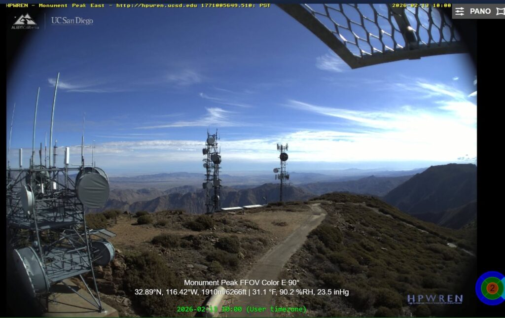
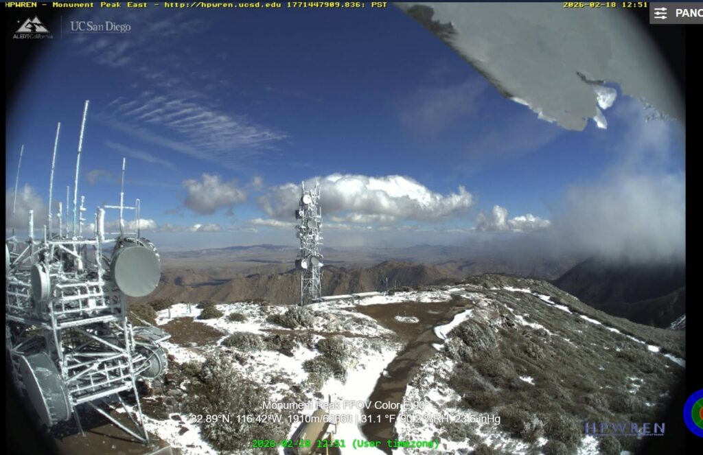

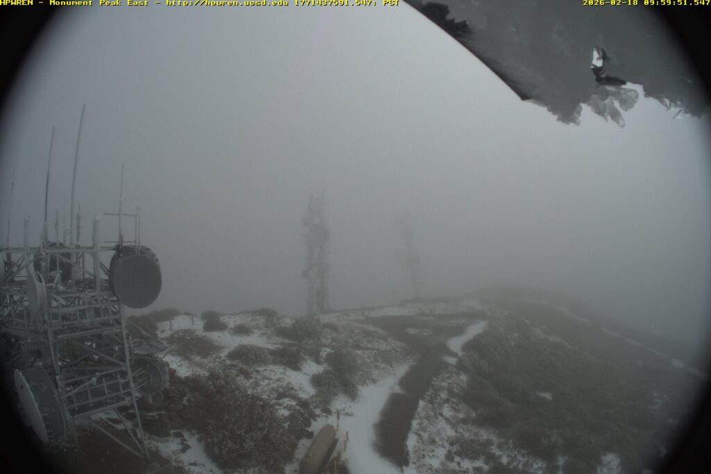
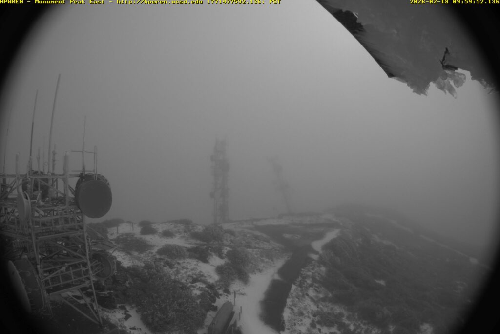
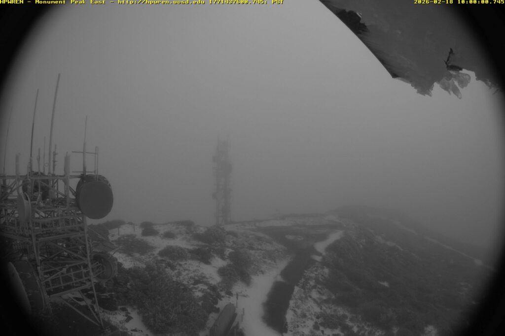
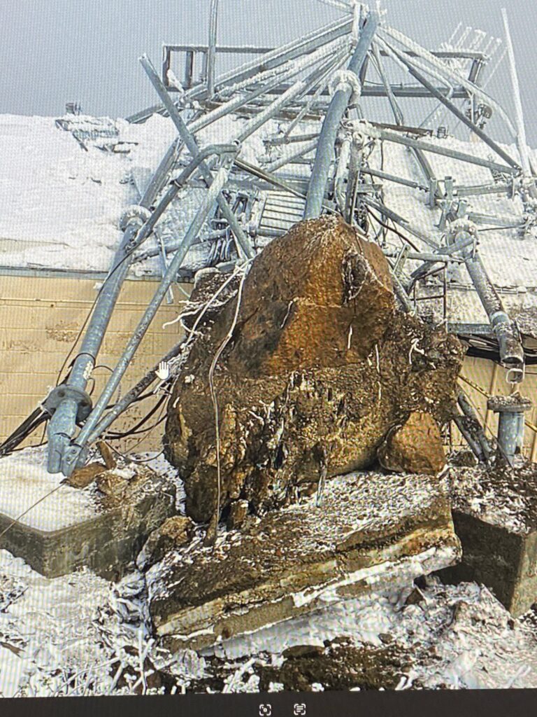
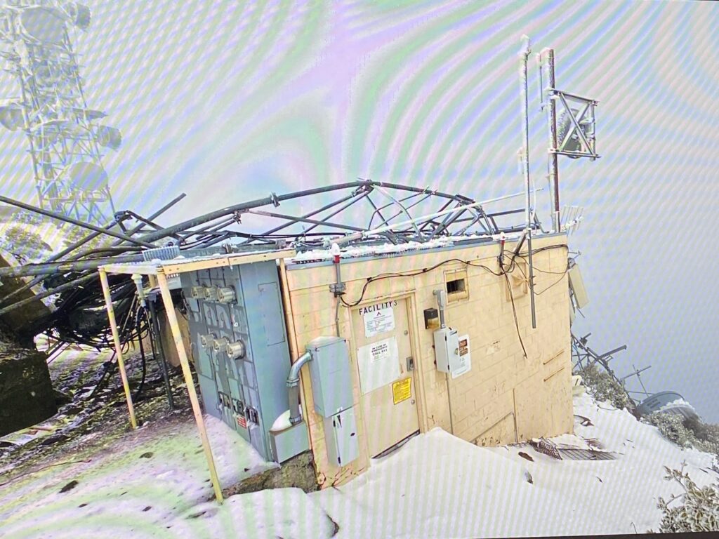
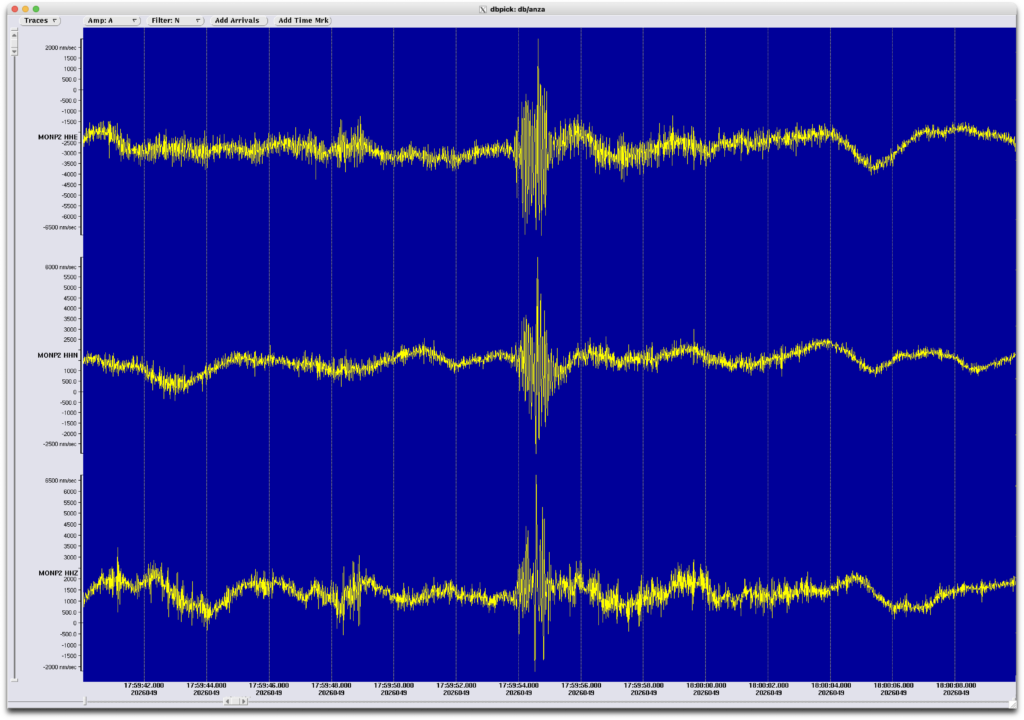
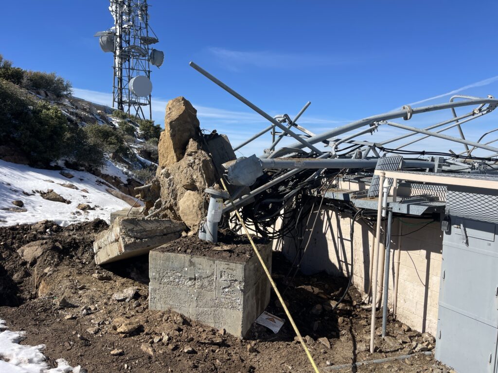
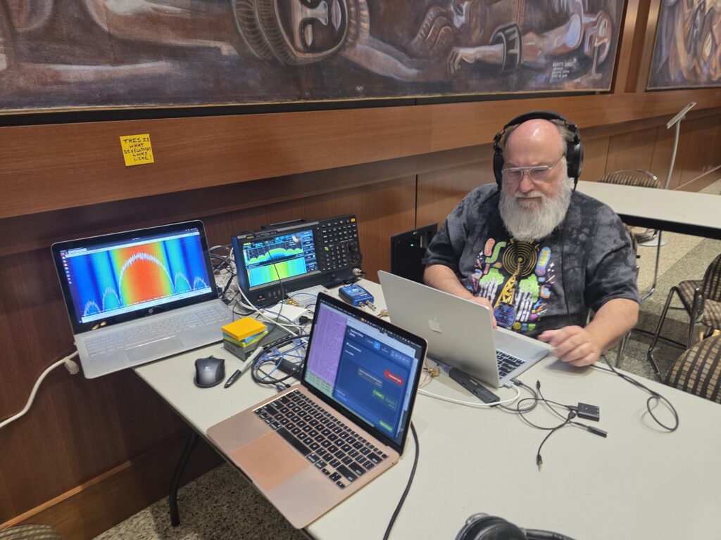
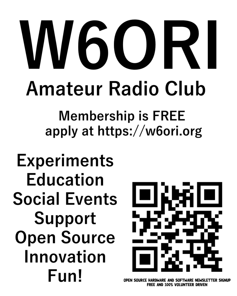

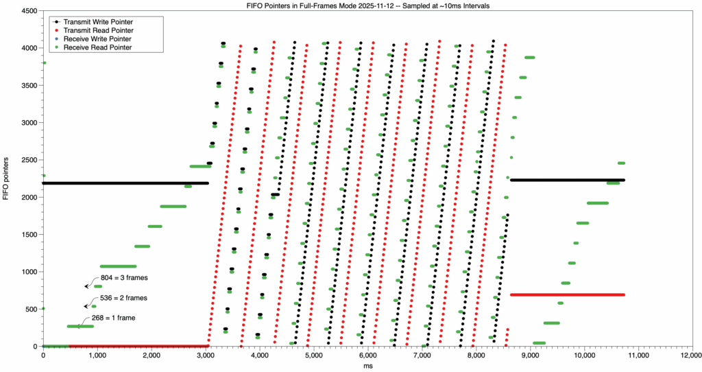
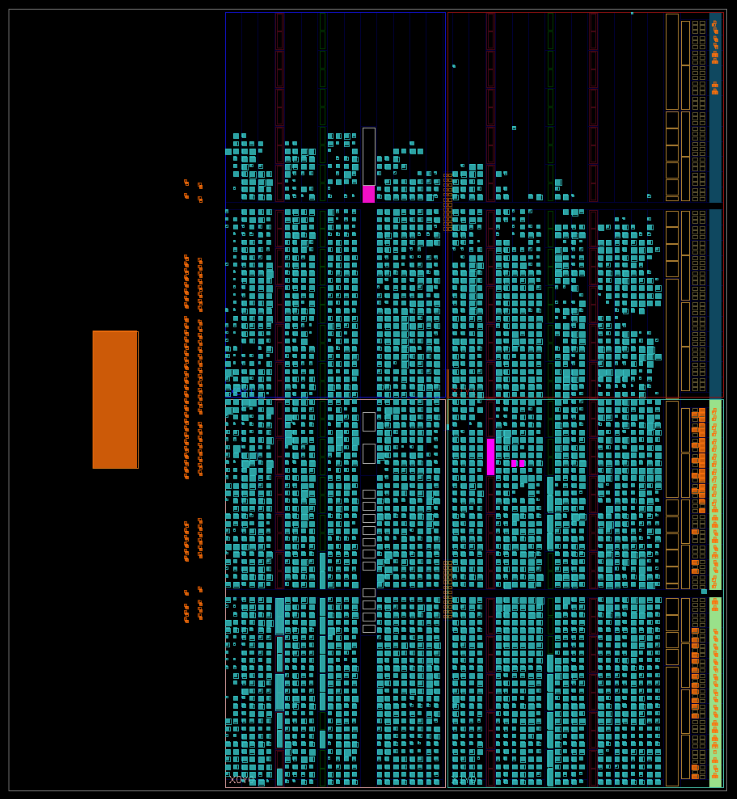
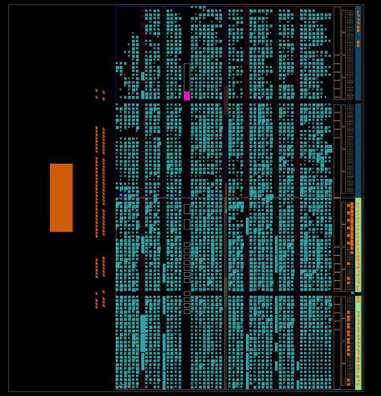
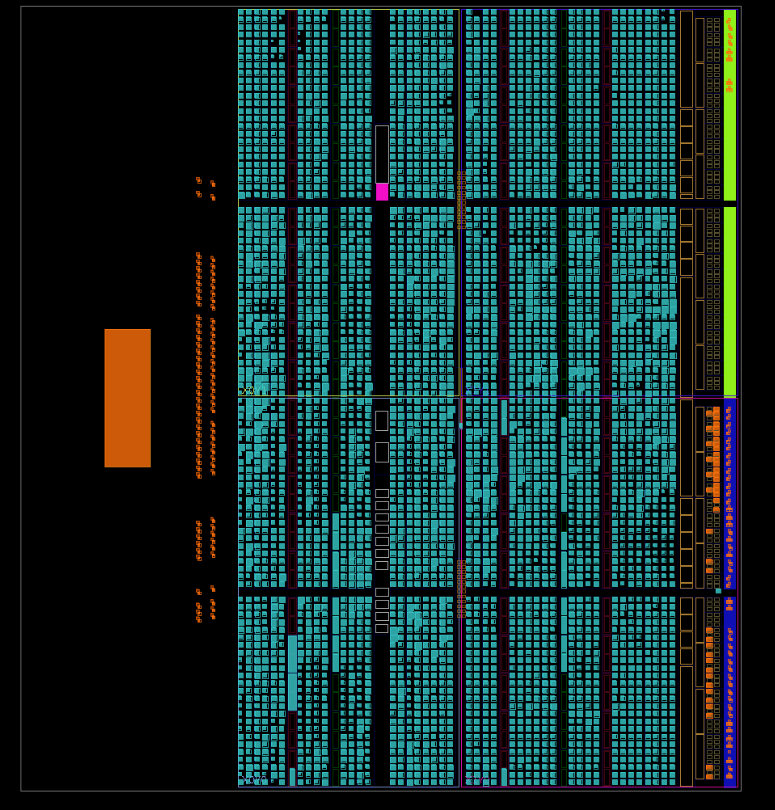
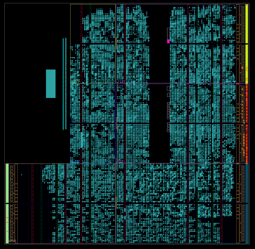
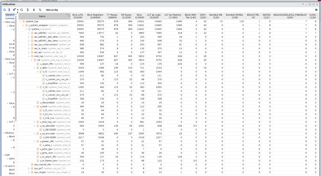
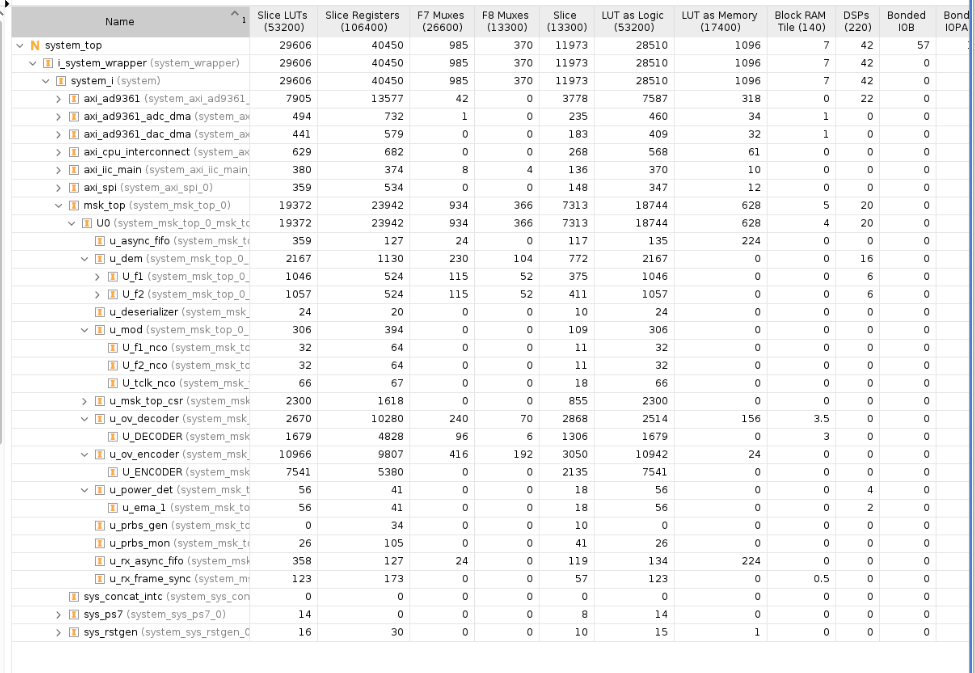
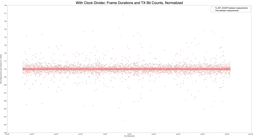
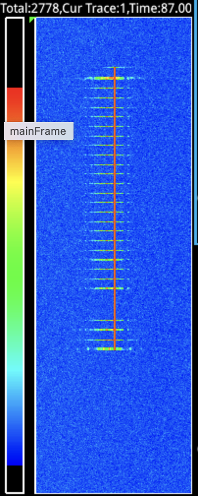
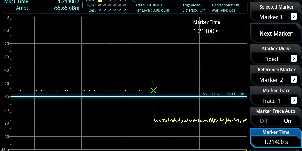
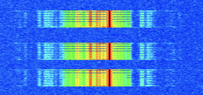
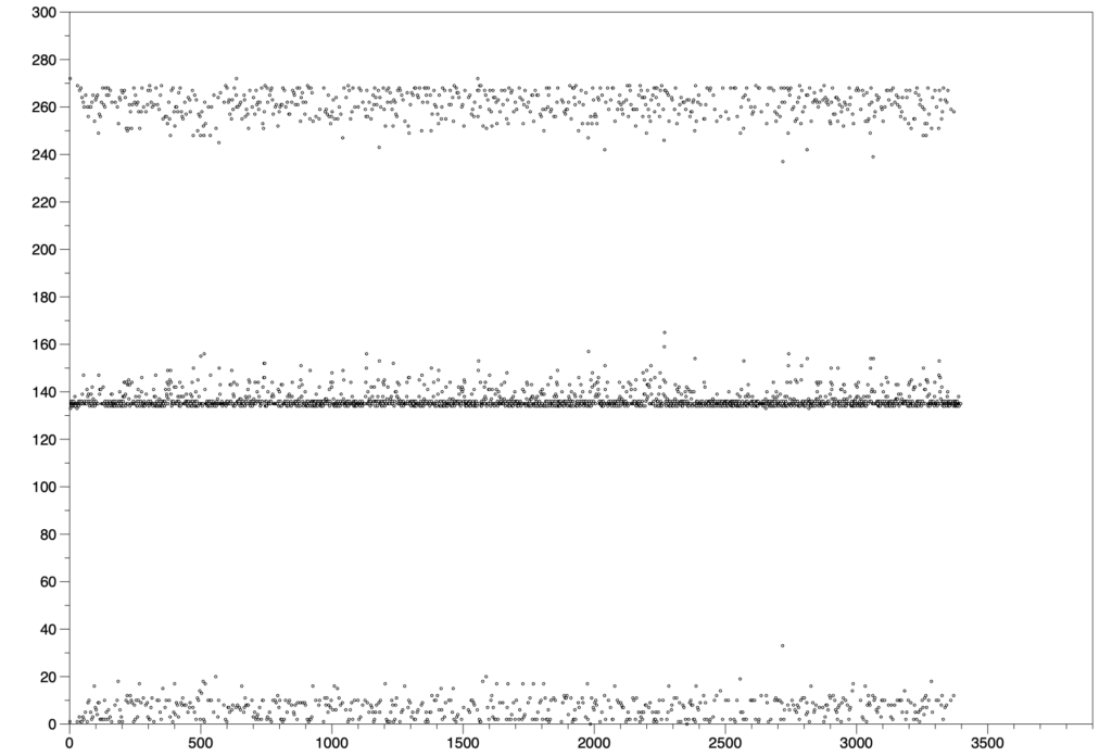
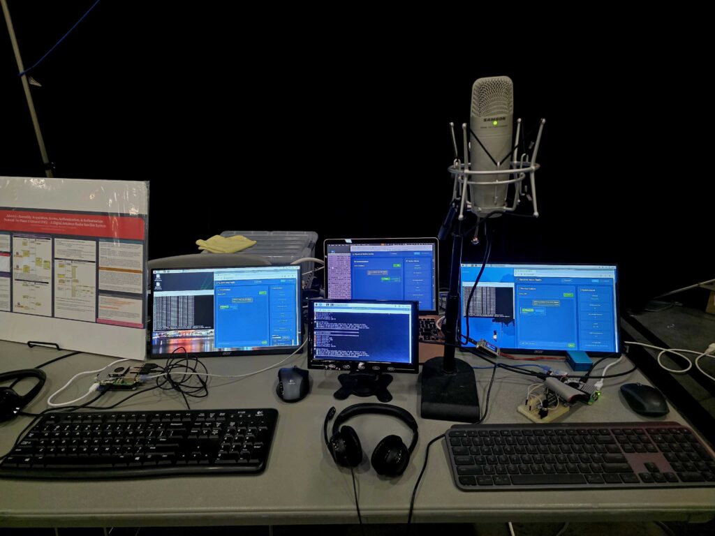
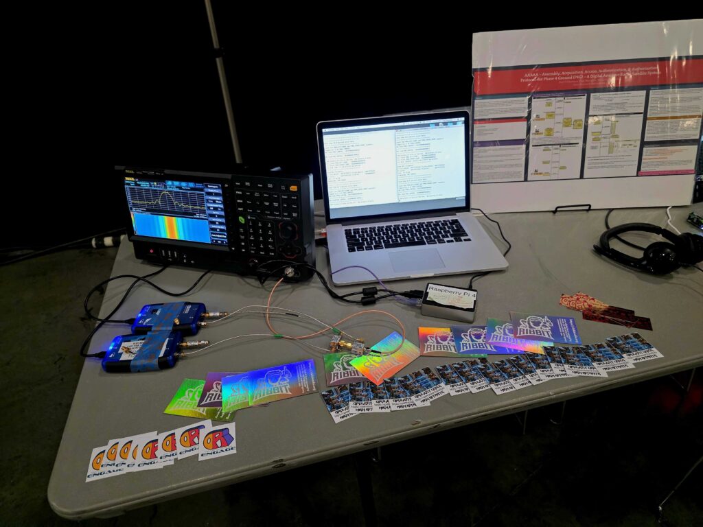
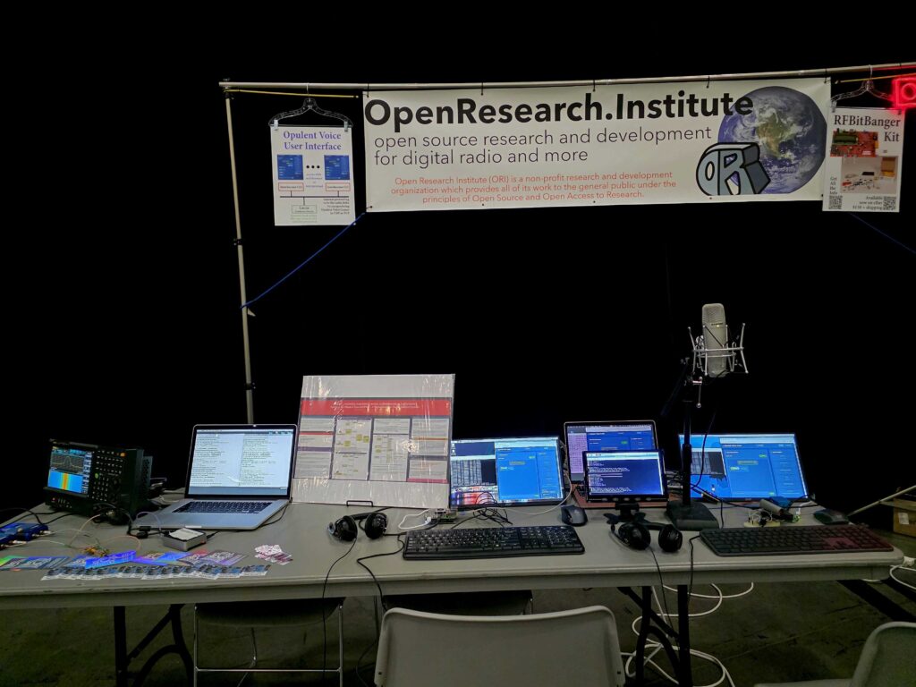
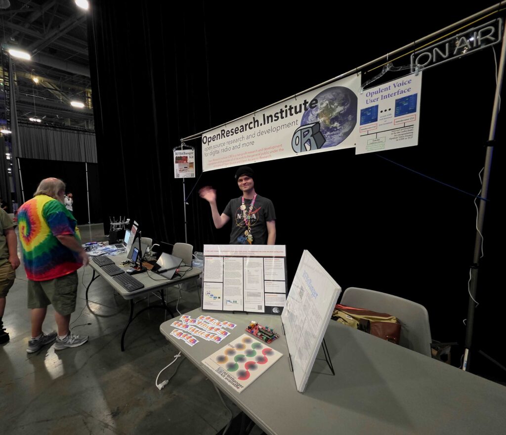
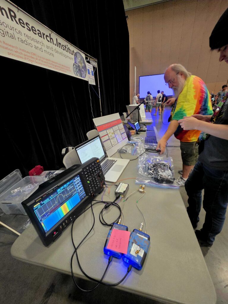

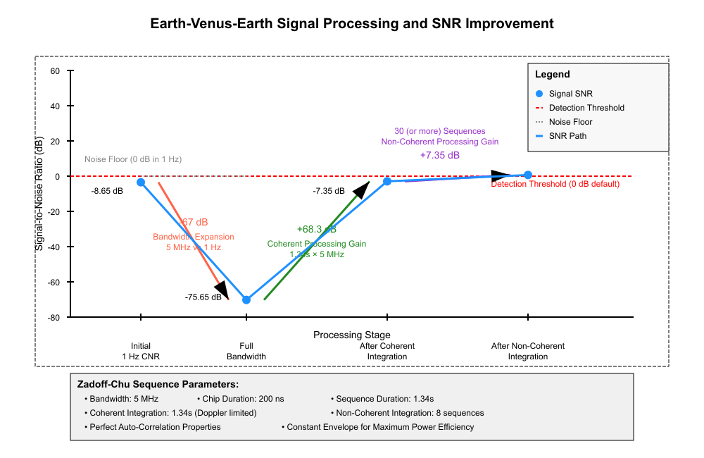
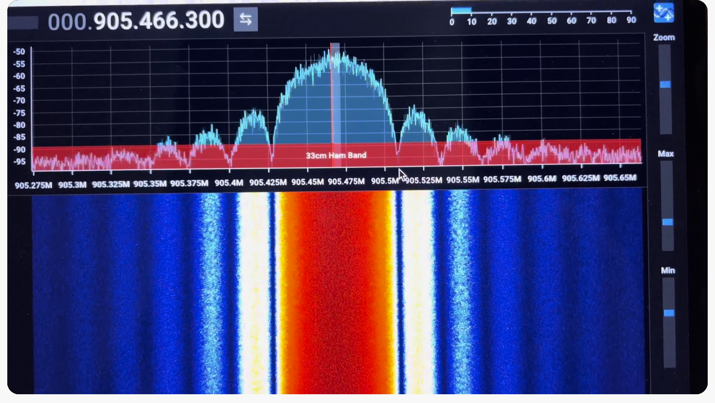
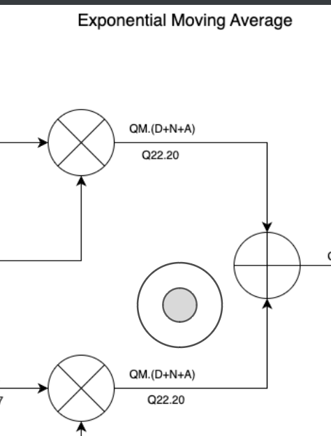


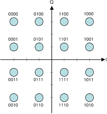
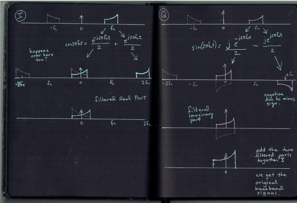
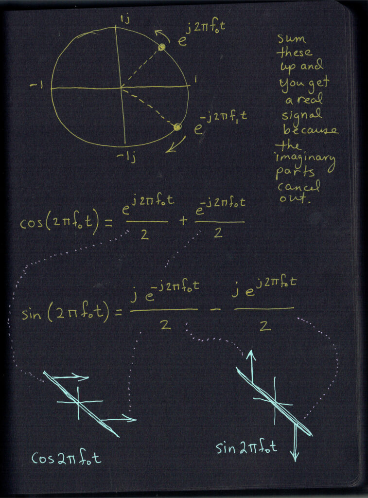
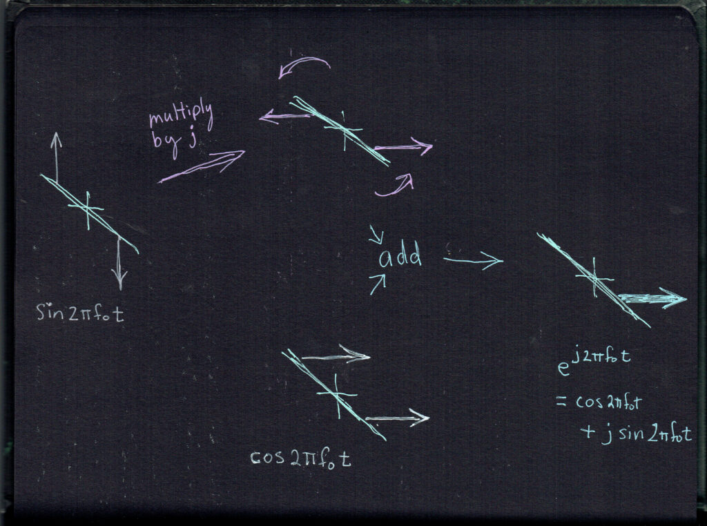
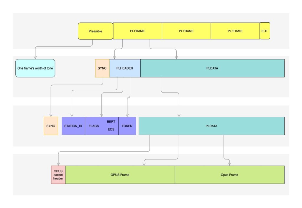
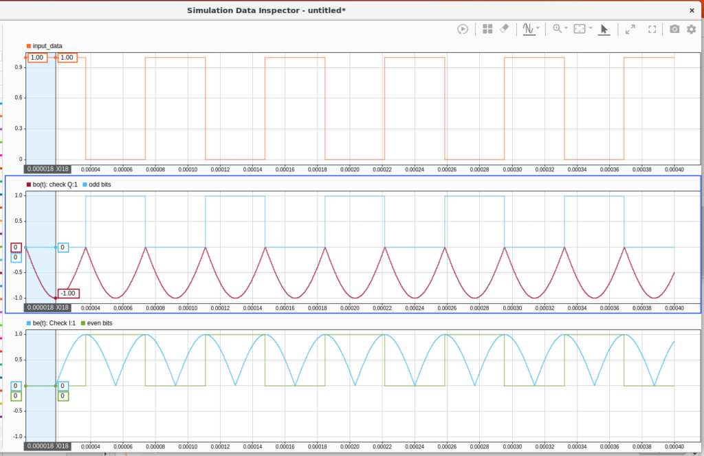
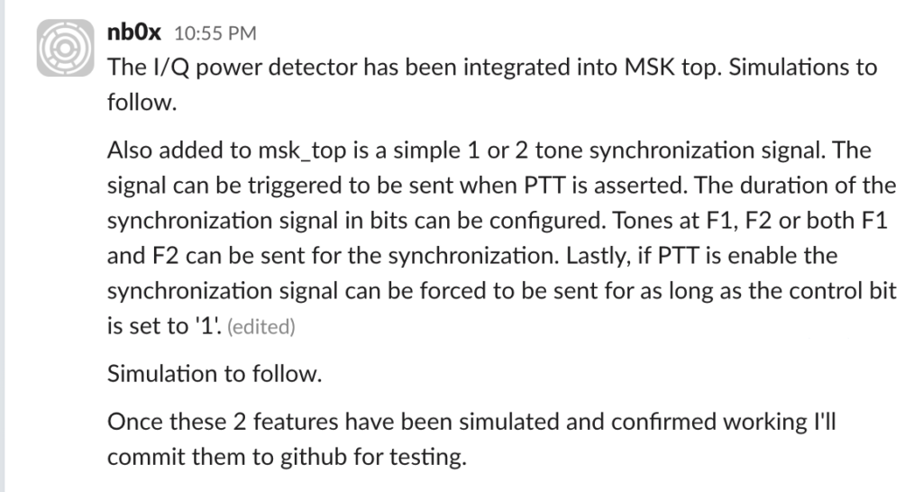

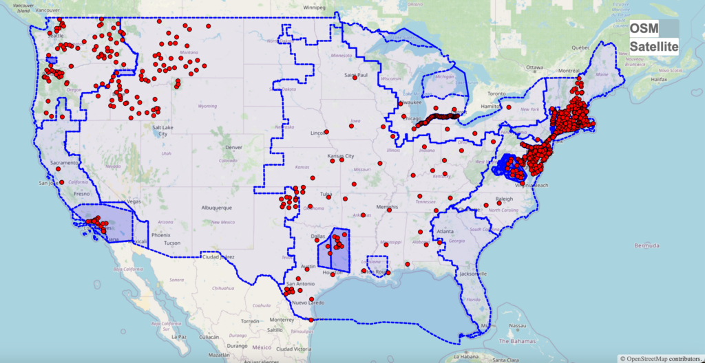
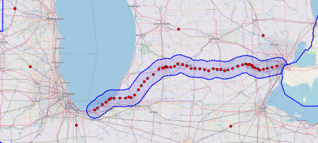
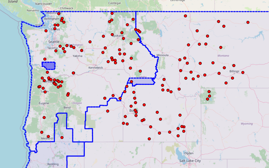

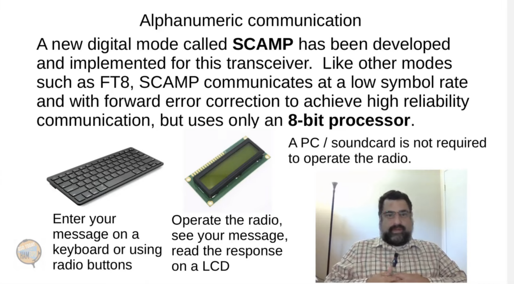


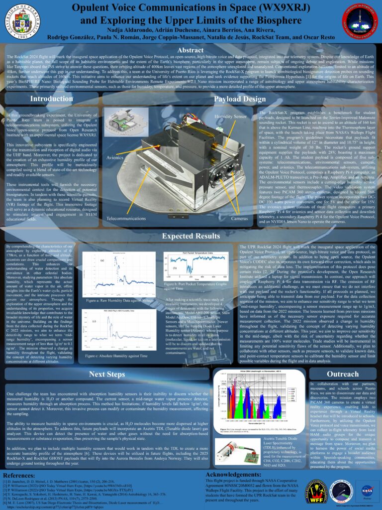
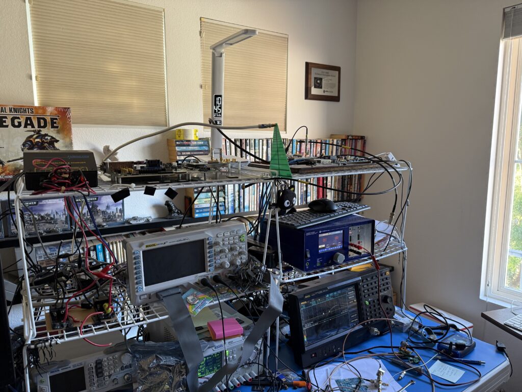
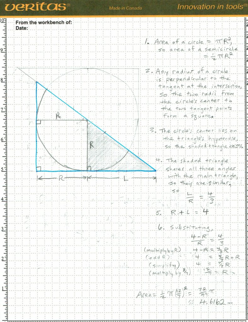
 Amaranth