With receiver data successfully collected by Dwingeloo and Stockert amateur radio astronomy sites during the Earth-Venus-Earth communications event on 22 March 2025, attention moved to processing the data to see if the transmitted carrier wave signal could be detected.
Four transmissions of a carrier wave from the Dwingeloo radio astronomy site were made. Each transmission was 278 seconds long. This time span was selected because it equaled the expected round-trip time from Earth to Venus and back. This would allow the transmitter to transmit for the round trip time, shut down, and then immediately begin receiving what should be the leading edge of the reflected radio signal. Both Dwingeloo and Stockert made time-coordinated in-phase and quadrature (IQ) recordings of the receive spectrum.
IQ samples are complex numbers that are created by sampling a received waveform. IQ samples fully specify any waveform, as long as they are taken at a rate faster than twice the bandwidth of the recorded signal. These IQ time series recordings are then mathematically evaluated in order to reveal the reflected carrier wave spike in the frequency domain.
Raw data (at 1 MSps), decimated data (at 5 kSps), and an example data processing Python Notebook are available from https://data.camras.nl/venus/
The data files are in SigMF format. This format is widely used for IQ signal data recordings. A data file, containing IQ samples, is paired with a metadata file, which has a variety of metadata describing the conditions and configurations of recorded data. Learn more about SigMF at https://sigmf.org
In addition to the SigMF files and a Python Notebook that performs the data analysis, there are also two comma separated value (CSV) files containing the expected frequency offsets and Doppler rates for RX timestamps. There is one for Stockert and one for Dwingeloo. These values are needed by the script in order to correct the received samples frequency shifts due to Doppler.
Once the notebook eve-cw-detect-example.ipynb is downloaded from the site, then all of the 5 kSps files, dwingeloo_venus_doppler.csv and stockert_venus_doppler.csv should also be downloaded.
While the 1 MSps files are higher resolution, the 5 kSps files are more than enough resolution to carry out the math. It takes much less time to process these smaller lower resolution files than the larger higher resolution files, and the results will be exactly the same.
Note: There is a bug in the python package sigmf version 1.2.8 that prevents these files from loading. Please install 1.2.6 or a version greater than 1.2.8. Or, modify the script to set up a SigMFFile instace manually, to evade the bug.
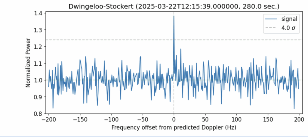
Run the script, and if all goes well, the visualization will show a spike for the carrier wave. Success!
What is this script doing?
Here is a summary of the most important calculations.
The notebook loads the recorded IQ data SigMF files and the Doppler information from CSV files. It then compensates for both the Doppler shift and Doppler rate of change using phase rotation.
# Compensate for Doppler and Doppler rate
dr = np.repeat(doppler_rate, len(data) / len(doppler_rate))
t_s = np.arange(len(data)) / fs
fdrift = -dr # Doppler rate
f0_Hz = -expected_freq_offset # Doppler
phi_Hz = (fdrift * t_s**2) / 2 + (f0_Hz * t_s) # Instantaneous phase.
phi_rad = 2 * np.pi * phi_Hz # Convert to radians.
data = data * np.exp(1j * phi_rad)
This means our signal will be centered at 0 Hz offset for the rest of the processing.
Next, we do some coherent processing. Coherent processing means that we preserve the phase information of the signal. Non-coherent processing just looks at the amplitude. Fast Fourier Transforms (FFT) preserve magnitude and phase.
spectrum = np.fft.fftshift(np.fft.fft(data.reshape(-1, int(sample_rate))))
The data is reshaped to have segments of length sample_rate (which is 5000 samples per second), meaning each FFT operation is performed on exactly 1 second of data. This is the coherent integration time used in the experiment.
This is less than the maximum coherency time available due to Doppler rate of change limitations (~1.3 seconds), but it is larger than another maximum limit due to Doppler Spread from Venus’ rotation (we calculated a much lower 0.03 seconds based on 31 Hz). The reasoning for being able to use 1 second coherent integration time (based on a Doppler Spread of 1Hz) is that the updated Doppler Spread is not as bad as we originally calculated.
After obtaining the FFT results, the notebook performs non-coherent integration by averaging the magnitudes of the FFT outputs. This means it discards the phase information and combines power/energy over the entire recording run.
spec_sum = np.mean(np.abs(spectrum), axis=0)
The axis=0 parameter means it’s averaging across multiple 1-second segments, effectively performing non-coherent integration over the entire 278 second long recording duration. This allows us to integrate over much longer periods than would be possible with purely coherent integration.
Dwingeloo’s Thomas Telkamp invites the community to expand on and improve the Python notebook, saying in late March 2025, “A few remarks: 1) use the 5ksps files, 2) there is an example notebook now on how to process the data, and 3) you’re not supposed to duplicate it, but to improve it!”
Also, please read the excellent analysis from Dr. Daniel Estevez at https://destevez.net/2025/04/analysis-of-the-camras-venus-radar-experiment/
And, additional details from Cees Bassa can be found at https://www.camras.nl/en/blog/2025/first-venus-bounce-with-the-dwingeloo-telescope/
One Reply to “How to Process an Earth-Venus-Earth Radar Return Signal”