Month: December 2025

This article documents the process of upgrading a working hard-decision Viterbi decoder to soft-decision decoding in an FPGA-based MSK modem implementing the Opulent Voice protocol. Soft-decision decoding provides approximately 2-3 dB of coding gain over hard-decision, which is significant for satellite communications and weak signal work where every dB matters. We describe the architectural changes, the bugs encountered, and the systematic debugging approach used to resolve them.

Introduction

The Opulent Voice (OPV) protocol uses a rate 1/2, constraint length 7 convolutional code with generator polynomials G1=171 and G2=133 in octal representation. The original implementation used hard-decision Viterbi decoding, where each received bit is quantized to 0 or 1 before decoding. Soft-decision decoding preserves additional information from the demodulator. In addition to the output of a 0 or a 1, we also have what we are going to call “confidence information” from the demodulator. This additional information allows us to make better decisions because some bits are more reliable than others. Some bits come in strong and clear and others are very noisy. If we knew how sure we were about whether the bit was a 0 or a 1, then we could improve our final answers on what we thought was sent to us. How is this improvement achieved? We can’t read the mind of the transmitter, so where does this “confidence information” come frome? How do we use it?

Consider receiving two bits. We get one bit with a strong signal and we get the other bit near the noise floor. Hard decision treats both bits equally. They’re either 0 or 1, case closed. Soft decision decoding says “I’m 95% confident this first bit is a 1, but only 55% confident about the second bit being a 0.” When the decoder must choose between competing paths, it can weight reliable bits more heavily than the ones it has less confidence about.

When our modem demodulates a bit, the result is calculated as a signed 16 bit number. For hard decisions, we just take the sign bit from this number. This is the bit that tells us if the number is positive or negative. Negative numbers are interpreted as 1 and positive numbers are interpreted as 0. The rest of the number, for hard decisions, is thrown away. However, we are going to use the rest of the calculation for soft decisions. How close to full scale 1 or 0 was the rest of the number? This is our confidence information.

In practice, a technique called 3-bit soft quantization captures most of the available information and gets us the answers we are after. Quantization means that we translate our 16 bit number, which represents a very high resolution of 65536 levels of confidence, into a 3 bit number, which represents a more manageable 8 levels of confidence. Think of this like when someone asks you to rate a restaurant on a scale from 1 to 5. That’s relatively easy. 1 is terrible. 5 is great. 3 is average, or middle of the road. If you were asked to rate a restaurant on a scale from 1 to 65536, you probably could, but how many levels of quality are there really? Simplifying a rating to a smaller number of steps makes it easier to deal with and communitcate to others. This is what we are doing with our 16 bit calculation. Converting it to a 3 bit calcuation simplifies our design by quite a bit without sacrificing a lot of performance. We can always go back to the 16 bit number if we have to. Since we were using signed binary representation, 000 is the biggest number and 111 is the smallest. If we print the numbers out, you can see how it works if we just take the sign bit and “round up” or “round down” the rest of the result.

Here’s our quantized demodulator output. The sign of the number (positive or negative) is the first binary digit. Then the rest of the number follows.

000 largest positive number - definitely received a 0
001 probably a 0
010 might be a 0
011 close to zero, but still positive
100 close to zero, but still negative
101 might be a 1
110 probably a 1
111 smallest negative number - definitely received a 1

After the conversion, our implementation uses the following rubric.

confidence        outcome
000               strong ‘0’ (high positive correlation)
111               strong ‘1’ (high negative correlation)
011-100           uncertain!

System Architecture

Original Hard-Decision Path

[Demodulator] to [Frame Sync] to [Frame Decoder] to [Output]
                     |              |
                  rx_bit      Deinterleave
                  rx_valid    Hard Decision Viterbi
                              Derandomize

The hard-decision path is as follows. The demodulator outputs `rx_bit` (0 or 1) and an `rx_valid` strobe. This strobe tells us when the `rx_bit` is worth looking at. We don’t want to pick up the wrong order, or get something out of the oven too early (still frozen) or too late (oops it’s burned). `rx_valid` tells us when it’s “just right”.  The frame sync detector finds sync words in the incoming received bitstream and then assembles bytes into frames. The sync word is then thrown away, having done its job. The resulting frame needs to be deinterleaved, to put the bits back in the right order, and then we do our forward error correction. After that, we derandomize. We now have a received data frame.

New Soft-Decision Path

[Demodulator] to [Frame Sync Soft] to [Frame Decoder Soft] to [Output]
                     |                      |
                  rx_bit              Deinterleave
                  rx_valid            Soft Decision Viterbi
                  rx_soft[15:0]       Derandomize
                     |
              Quantize to 3-bit
              Store soft buffer

There is a lot here that is the same. We deinterleave, decode, and derandomize. We decode with a new soft decision Viterbi decoder, but the flow in the soft frame decoder is essentially the same as in the hard decision version.

What is new is that the demodulator provides 16-bit signed soft metric alongside the previously provided hard bit. This is just bringing out the “rest” of the calculation used to get us the hard bit in the first place. A really nice thing about our radio design is that this data was there all along. We didn’t have to change the demodulator in order to use it.

Another update is that the frame sync detector quantizes and buffers these soft “confidence information” values. So, we have an additional buffer involved. Finally, the frame decoder uses soft Viterbi with separate G1/G2 soft inputs, instead of the `rx_bit` that we were using before.

Implementation Details

Soft Value Quantization

The demodulator’s soft output is the difference between correlator outputs: `data_f1_sum – data_f2_sum`. Large positive values indicate confident ‘0’, large negative indicate confident ‘1’.

FUNCTION quantize_soft(soft : signed(15 DOWNTO 0)) RETURN std_logic_vector IS
BEGIN
    -- POLARITY: negative soft = ‘1’ bit, positive soft = ‘0’ bit
    IF soft < -300 THEN
        RETURN “111”;  -- Strong ‘1’ (large negative soft)
    ELSIF soft < -150 THEN
        RETURN “101”;  -- Medium ‘1’
    ELSIF soft < -50 THEN
        RETURN “100”;  -- Weak ‘1’
    ELSIF soft < 50 THEN
        RETURN “011”;  -- Erasure/uncertain
    ELSIF soft < 150 THEN
        RETURN “010”;  -- Weak ‘0’
    ELSIF soft < 300 THEN
        RETURN “001”;  -- Medium ‘0’
    ELSE
        RETURN “000”;  -- Strong ‘0’ (large positive soft)
    END IF;
END FUNCTION;

The thresholds (+/- 50, +/- 150, +/- 300) must be calibrated for the specific demodulator. If you want to implement our code in your project, then start with these values and adjust based on observed soft value distributions.

Soft Buffer Architecture

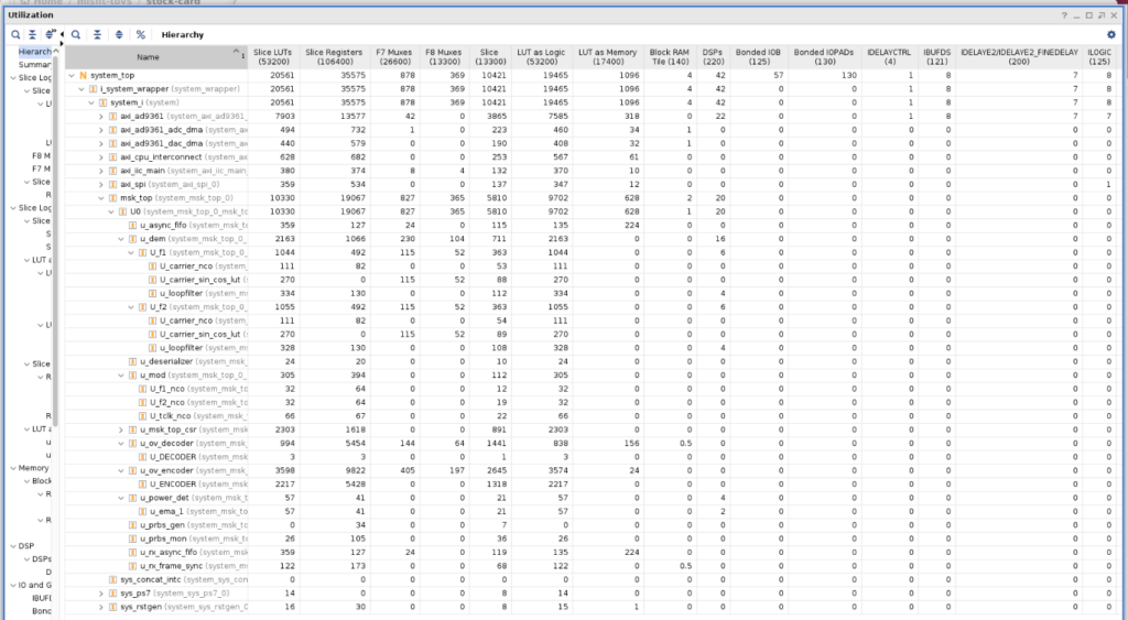
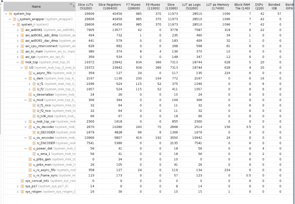
The Opulent Voice frame contains 2144 encoded bits (134 payload bytes × 8 bits × 2 for rate-1/2 error correcting code). Each bit needs a 3-bit soft value, requiring 6432 bits of storage.

TYPE soft_frame_buffer_t IS ARRAY(0 TO 2143) OF std_logic_vector(2 DOWNTO 0);
SIGNAL soft_frame_buffer : soft_frame_buffer_t;

Bit Ordering Challenges

The most subtle bugs in getting this design to work involved bit ordering mismatches between hard and soft paths. The system has multiple bit-ordering conventions that must align. There were several bugs that tripped us up in this category. The way to solve it was to carefully check the waveforms and repeatedly check assumptions about indexing.

Byte transmission: MSB-first (bit 7 transmitted before bit 0)
Byte assembly in receiver: Shift register fills MSB first
Interleaver: 67×32 matrix, column-major order
Soft buffer indexing: Must match hard bit indexing

The Arrival Order Problem

Bytes transmit MSB-first, meaning for byte N a `bit_count` of 0 receives byte(7) = interleaved[N×8 + 7] and a `bit_count` of 7 receives byte(0) = interleaved[N×8 + 0]

The hard path naturally handles this through shift register assembly. The soft path must explicitly account for it. We got this wrong at first and had to sort it out carefully.

Wrong approach which caused bugs:

-- Tried to match input_bits ordering with complex formula
soft_frame_buffer(frame_byte_count * 8 + (7 - bit_count)) <= quantize_soft(...);

This formula has a timing bug: `bit_count` is read before it updates (VHDL signal semantics), causing off-by-one errors.

Correct approach which gave the right results:

-- Store in arrival order, handle reordering in decoder
soft_frame_buffer(frame_soft_idx) <= quantize_soft(s_axis_soft_tdata);
frame_soft_idx <= frame_soft_idx + 1;

Then in the decoder, we used a combined deinterleave+reorder function:

FUNCTION soft_deinterleave_address(deint_idx : NATURAL) RETURN NATURAL IS
    VARIABLE interleaved_pos : NATURAL;
    VARIABLE byte_num : NATURAL;
    VARIABLE bit_in_byte : NATURAL;
BEGIN
    -- Find which interleaved position has the deinterleaved bit
    interleaved_pos := interleave_address_bit(deint_idx);
    -- Convert interleaved position to arrival position (MSB-first correction)
    byte_num := interleaved_pos / 8;
    bit_in_byte := interleaved_pos MOD 8;
    RETURN byte_num * 8 + (7 - bit_in_byte);
END FUNCTION;

Soft Viterbi Decoder

The soft Viterbi decoder computes branch metrics differently than hard Viterbi decoders. Hard-decision branch metric has a Hamming distance of 0, 1, or 2.

branch_metric := (g1_received XOR g1_expected) + (g2_received XOR g2_expected);

Soft-decision branch metric is the sum of soft confidences.

-- For expected bit = ‘1’: metric = soft_value (high if received ‘1’)
-- For expected bit = ‘0’: metric = 7 - soft_value (high if received ‘0’)
IF g1_expected = ‘1’ THEN
    bm := bm + unsigned(g1_soft);
ELSE
    bm := bm + (7 - unsigned(g1_soft));
END IF;
-- Same for G2

The path with the highest cumulative metric wins. This is the opposite convention from hard-decision Hamming distance, where the least differences between two different possible patterns wins.

Debugging Journal

Bug #1: Quantization Thresholds

Symptom was all soft values were 7 (strong ‘1’). But, we knew our data was about half 0 and about half 1. The root cause was that initial thresholds (+/- 12000) were far outside the actual soft value range (+/- 400). We adjusted thresholds to +/- 300, +/- 150, and +/- 50.

Lesson? Always check actual signal ranges before setting thresholds.

Bug #2: Polarity Inversion

Symptom was that output frames were bit-inverted. The root cause was that soft value polarity convention was backwards?positive was mapped to ‘1’ instead of ‘0’. This was fixed by inverting the quantization mapping.

Bug #3: Viterbi Output Bit Ordering

The symptom was that decoded bytes had reversed bit order. Viterbi traceback produces bits in a specific order that wasn’t matched during byte packing. After several missed guesses, we corrected the bit-to-byte packing loop.

FOR i IN 0 TO PAYLOAD_BYTES - 1 LOOP
    FOR j IN 0 TO 7 LOOP
        fec_decoded_buffer(i)(j) <= decoder_output_buf(PAYLOAD_BYTES*8 - 1 - i*8 - j);
    END LOOP;
END LOOP;

Bug #4: VHDL Timing – Stale G1/G2 Data

The symptom was that the first decoded bytes were correct, and the rest were garbage. This was super annoying. The root cause was that `decoder_start` was asserted in the same clock cycle as G1/G2 packing, but VHDL signal assignments don’t take effect until process end. We added pipeline stage. We pack G1/G2 in `PREP_FEC_DECODE`, assert start, and wait for `decoder_busy` before transitioning to `FEC_DECODE`

Bug #5: Vivado Optimization Removing Signals

In Vivado’s waveform visualizer, the `deinterleaved_soft` array was partially uninitialized in simulation. The cause was unclear, but we surmised that Vivado optimized away signals it deemed unnecessary.

We added `dont_touch` and `ram_style` attributes. This seemed to fix the symptom, but we didn’t feel like it was a cure.

ATTRIBUTE ram_style : STRING;
ATTRIBUTE ram_style OF soft_buffer : SIGNAL IS “block”;
ATTRIBUTE dont_touch : STRING;
ATTRIBUTE dont_touch OF soft_buffer : SIGNAL IS “true”;

Bug #6: Soft Buffer Index Timing

We saw that soft values were stored at wrong indices. The entire pattern was shifted. Storage formula `byte*8 + (7 – bit_count)` read `bit_count` before increment, which pulled everything off by one. Waveform showed index 405 being written when 404 was expected. The formula was mathematically correct, but VHDL signal assignment semantics meant `bit_count` had its old value.

We abandoned the complex indexing formula. We now store in arrival order using simple incrementing counter and handle reordering in decoder.

Bug #7: Wrong Randomizer Sequence

Output frames were completely corrupted despite all other signals appearing correct. The cause was that the soft decoder was created with a different randomizer lookup table than the encoder and hard decoder.

Encoder/Hard Decoder: `x”A3”, x”81”, x”5C”, x”C4”, …`
Soft Decoder (wrong): `x”96”, x”83”, x”3F”, x”5B”, …`

When creating the soft decoder, the randomizer table was generated incorrectly instead of being copied from the working hard decoder. We copied exact randomizer sequence from `ov_frame_decoder.vhd`, and it started working. Lesson learned? When creating a new module based on an existing one, copy constants exactly. Don’t regenerate them.

Debugging Methodology

Systematic Signal Tracing

When output is wrong, work backwards from output to input. Check final output values. Check intermediate values after major transformations (after derandomize, after Viterbi, after deinterleave). Check input values to each stage, even if you totally believe you’re getting the right data. Find where expected and actual diverge. Don’t try to solve “in the middle” of wrongness. Work on finding the edges between correct and incorrect, even if it points in unexpected directions.

Reference Implementation

Maintain a reference design. This independent design needs to be different than the platform and language that you are working on. This reference performs identical operations and can help you figure things out. For example, our Python references helped us solve problems in our VHDL.

def convolutional_encode(input_bits):
    G1, G2 = 0o171, 0o133
    shift_reg = 0
    output = []
    for bit in input_bits:
        shift_reg = ((shift_reg << 1) | bit) & 0x7F
        g1_bit = bin(shift_reg & G1).count(‘1’) % 2
        g2_bit = bin(shift_reg & G2).count(‘1’) % 2
        output.extend([g1_bit, g2_bit])
    return output
def interleave(bits):
    ROWS, COLS = 67, 32
    interleaved = [0] * len(bits)
    for i in range(len(bits)):
        row, col = i // COLS, i % COLS
        interleaved[col * ROWS + row] = bits[i]
    return interleaved

Compare FPGA signals against reference at each stage.

Test Patterns

Use recognizable patterns that make errors obvious. For example, we use alternating frames for our test payload data. First frame is sequential. The bytes go 0x00, 0x01, 0x02, and so on up to 0x85. The second frame is offset from this. 0x80, 0x81, 0x82, up to 0xFF where it rolls over to 0x00, 0x01, 0x02,0x03, 0x04 ending at 0x05. Alternating distinctive frames like these help to reveal a wide variety of errors. Frame boundary issues, such as when a frame starts in the middle of another frame, can be spotted. Initialization issues might be revealed as the root cause if only first frame works and all the rest fail. And, state machine issues could be the underlying problem if the pattern of output bytes is inconsistent.

Waveform Analysis Tips

Check before clock edge! Signal values are sampled at rising edge. What you see “after” may be the next value, not the current value. Watch for ‘U’ (uninitialized). This indicates a signal never written or it got optimized away. Why wasn’t it ever written? Why is it missing? This is a clue! Track indices. When storing to arrays, verify both the index and value are correct. Off by one errors are very common. Compare parallel paths. If, for example, a hard decision path works but soft decisions do not, the difference reveals the bug.

Results

After fixing all bugs, the soft-decision decoder produces identical output to the hard-decision decoder for clean signals. The benefit appears at low SNR where soft decisions allow the Viterbi algorithm to make better path selections. Soft decisions add 2-3 additional dB of coding gain over hard decisions, which brought us 5 dB of coding gain.

Conclusions

Upgrading from hard to soft decision decoding requires careful attention to bit ordering, VHDL timing, polarity conventions, and code re-use. Multiple conventions must align. You have to get transmission order, assembly order, interleaver order, and buffer indexing all correct. Signal vs. variable semantics matter for single-cycle operations. This is a language-specific thing for VHDL, but all languages have crucial differences between the tools used to get things done in code. Document and verify positive/negative soft value meanings. In other words, pick heads or tails and stick with it. Copy constants and lookup tables exactly from working code. Re-use saves time until a copy and paste error slows the debugging process for hours or days.

The 2-3 dB coding gain from soft decisions is worth the implementation complexity for satellite communications where link margins are precious. The coding gain helps in terrestrial settings to increase range and reliability.

Source Code

The complete implementation is available in the Open Research Institute `pluto_msk` repository at `https://github.com/OpenResearchInstitute/pluto_msk`. `frame_sync_detector_soft.vhd` is the frame sync with soft value quantization and buffering. `ov_frame_decoder_soft.vhd` is the frame decoder with soft Viterbi. And `viterbi_decoder_k7_soft.vhd` is the soft-decision Viterbi decoder core. These are separate files from the hard decision versions, which are also available. Look for files without the soft in the titles. This work may still be in the encoder-dev branch when you read this, but the eventual destination is main.

Acknowledgments

This work was performed at Open Research Institute as part of the Opulent Voice digital voice protocol development. It is open source and is publised under CERN open hardware licesnse version 2.0. Special thanks to Paul Williamson KB5MU for Remote Labs hardware support and testing, Matthew Wishek NB0X for modem architecture, design, and implementation, and Evariste F5OEO for integration advice for the Libre SDR. Thank you to the many volunteers reviewing the work and providing encouragement and support during the debugging process.

The FCC’s “Delete, Delete, Delete” initiative proposes removing the entire Access Broadband over Power Line (BPL) regulatory framework (Part 15 Subpart G) from the Code of Federal Regulations. The reasoning: BPL was never successfully commercialized, so the rules are dead letter. This item is scheduled for the December 18, 2025 FCC Open Meeting.

For those who weren’t in the amateur radio trenches in the United States during the mid-2000s, BPL was one of the most contentious regulatory battles in recent ham radio history. The technology promised broadband internet delivery over power lines, but there was a big catch. Power lines make excellent antennas in the HF spectrum. BPL systems operating from 1.7 MHz to 80 MHz range caused substantial interference to amateur radio operations, shortwave broadcasting, and other licensed services. This was documented by radio groups large and small across the US. 

ARRL fought this battle all the way to federal court. In 2008, the DC Circuit Court found the FCC had violated the Administrative Procedure Act in its BPL rulemaking. At the time, this was recognized as a significant victory. The court ordered the FCC to reconsider, but the Commission largely reaffirmed its original rules in 2011, leading to continued legal challenges that seemed to promise to drag on for years. 

Then a plot twist happened. The market solved the problem before the courts got back around to it. Every major commercial BPL deployment in the United States eventually shut down because they failed their business cases. Fiber, DSL, cable, and wireless broadband simply won. The last significant BPL internet provider (IBEC) closed shop in 2012. Cincinnati’s BPL system pulled the plug in 2014.

Part 15 Subpart G contained special provisions for Access BPL devices, including things like exclusion zones, database registration requirements, consultation requirements, mandated measurement procedures, and notching requirements for amateur bands.

Without Subpart G, any future BPL-like device would be regulated under the general Part 15 unintentional radiator provisions. These are the same rules that govern everything from your laptop to your garage door opener.

So, does this matter now? Well, yes. First of all, good riddance. These rules governed a technology that no longer exists in commercial deployment. Removing dead regulations is good regulatory hygiene. If someone wanted to resurrect BPL tomorrow, they’d still need to meet Part 15 emission limits and couldn’t cause harmful interference to licensed services. That’s the spectrum regulatory reality regardless of Subpart G. But, it’s not that simple. The specialized Subpart G rules existed precisely because generic Part 15 limits were inadequate for dealing with how harsh BPL interference really was. NTIA studies showed that BPL systems operating at generic Part 15 limits had essentially 100% probability of interfering with nearby HF operations. Removing the framework means any future power-line broadband technology would start from scratch without the hard-won protections built into Subpart G.

This is being processed as what is known as a Direct Final Rule. This means that the FCC believes it’s non-controversial and doesn’t require the traditional notice-and-comment process. However, the agency is accepting input. If adverse comments are filed, the rule would convert to a standard rulemaking requiring public comment.

Parties who have views on this deletion (like ARRL, which invested significant resources fighting these battles) have an opportunity to weigh in before the December 18 meeting.

FCC Document: DOC-415572A1 (Delete, Delete, Delete – Direct Final Rule)
Current regulations: 47 CFR Part 15 Subpart G (§§15.601–15.615)  
Background: ARRL v. FCC, DC Circuit Court of Appeals (2008)

For ORI members interested in the regulatory history, the ARRL’s BPL archive at arrl.org/broadband-over-powerline-bpl contains extensive documentation of the interference measurements, court filings, and technical studies from this era.

BPL Regulatory Throwback

From ARRL Bulletin ARLB003, in February 2005:

ARRL CEO David Sumner, K1ZZ, called Powell’s performance ‘a deep disappointment’ after some initial optimism–especially given his unabashed cheerleading on behalf of the FCC’s broadband over power line (BPL) initiative.

‘It’s no secret that we thought Chairman Powell was going entirely in the wrong direction on BPL and dragging the other commissioners and FCC staff along–willing or not–because he was, after all, the chairman,’ Sumner said. ‘A new chairman might be a chance for a fresh start.’

When the FCC adopted new Part 15 rules for BPL last October, Powell called it ‘a banner day.’ While conceding that BPL will affect some spectrum users, including ‘all those wonderful Amateur Radio operators out there,’ Powell implied that the FCC must balance the benefits of BPL against the relative value of other licensed services.

How we went from theory to gates in optimizing the frame synchronization for Opulent Voice. 

Finding the beginning of a data frame in a noisy radio channel is like searching for a needle in a haystack. Except, the haystack is constantly shifting, and some of the hay looks suspiciously like needles. For the Opulent Voice digital voice protocol, we’ve tackled this physics challenge on two fronts. First, we mathematically optimized our synchronization word. Second, we upgraded our FPGA detector from hard-decision matching to soft-decision correlation in order to take advantage of the better mathematics of the optimized codeword.

When we first designed the frame structure for Opulent Voice, we experimented with a familiar tool used in legacy digital voice protocols, called Barker codes. These binary sequences, discovered by R.H. Barker in 1953, have near-perfect autocorrelation properties. This means that when you slide them past themselves, you get a sharp peak at alignment and minimal response elsewhere. The problem? The longest Barker code is only 13 bits, and we needed 24 bits. 

The textbook solution is concatenation. Lucky for us, we could stick an 11-bit Barker code together with a 13-bit Barker code, and get 24-bits output. This gives you 0xE25F35, with a Peak Sidelobe-to-Mainlobe Ratio (PSLR) of 3:1. Respectable, but we realized that this wasn’t necessarily optimal for 24 bits.

The answer required brute force. With 2^24 = 16,777,216 possible sequences, modern computers can exhaustively search the entire space in about 90 seconds. The results were illuminating. 6,864 sequences achieve the optimal PSLR of 8:1. This was nearly three times better than our concatenated Barker code.

We can think of this like antenna directivity. A PSLR of 8:1 means our “main lobe” (the correlation peak when perfectly aligned) is eight times stronger than any “sidelobe” (responses at other alignments). Higher PSLR translates directly to better false-detection rejection, especially in multipath environments where delayed signal copies can trigger spurious sync detections.

For Opulent Voice, we selected 0x02B8DB from the optimal set. Besides having the best possible PSLR, it has good DC balance (11 ones, 13 zeros) and a maximum run length of 6 zeros. This woulld be important for tracking loop stability in minimum shift keying modulation. The mnemonic is “oh to be eight dB” for the hex digits.

Having an optimal sync word is only half the battle. The detector implementation matters just as much.

Our original frame sync detector used Hamming distance. We counted up how many bits differed between the received pattern when compared to our known sync word. If fewer than some threshold differ, we declared that sync was found. This works fine for strong signals, but there’s a fundamental problem buried lower in the noise. By the time bits reach the detector, the minimum shift keying demodulator has already made “hard decisions”. That means that each symbol has been quantized to a definitive 0 or 1. 

Hard decisions throw away valuable information. The demodulator might have been 99% confident about one bit but only 51% confident about another, yet both become equally weighted in the Hamming distance calculation. In a D&D analogy, it’s like reducing your attack rolls to just “hit” or “miss” without tracking the actual roll. You lose the ability to distinguish a near-miss from a catastrophic fumble. Now, if all we had to work with was hard decisions, then this is the best we could do. But there’s something really neat about our demodulator. It also decodes how confident is is of that 1 or 0. The soft decision metric is already produced and already available as a demodulator output.

The solution to our sync word detection optimizaiton problem is to use soft-decision correlation. Instead of binary bits, we work with signed values that indicate both the decision and the confidence. A value of +7 means “definitely a 0 with high confidence,” while +1 means “probably a 0 but not very sure.” Negative values indicate 1s.

The math is elegant. For each of the 24 sync word positions, we multiply the soft sample by +1 if we expect a ‘0’ or -1 if we expect a ‘1’, then sum all 24 products. Perfect alignment produces a large positive value; misalignment produces values near zero. The peak stands out sharply from the noise floor. We already had the information. We just had to use it.

The new `frame_sync_detector.vhd` in our encoder-dev branch implements soft-decision correlation with several key features:

First, we have parallel data paths. We maintain two shift registers. One is for soft decisions (24 × 16-bit signed values) and one is for hard decisions (24 bits). The soft path feeds the correlator; the hard path handles byte assembly after sync is found. This lets us have our cake and eat it too.

Second, we have polarity-aware correlation. This sounds fancy, but it’s a simple process. Our minimum shift keying demodulator uses a convention where positive soft values indicate ‘0’ bits and negative values indicate ‘1’ bits. The correlator accounts for this. When the sync word expects a ‘1’, we subtract the sample (making a negative contribution become positive). This detail matter. If we get the polarity wrong then our correlator becomes an anti-correlator.

Third, we have frame tracking with a flywheel. Once locked, we don’t search for sync on every bit. Instead, we count through the known frame length and verify sync where we expect it. This “flywheel” approach dramatically reduces computation and provides robustness against brief interference. We maintain lock through up to two consecutive missed syncs before returning to full search mode.It takes three consecutive successful sync word detections to declare lock. We may update these numbers later on if they are too small or too big. This is a good start and is similar to what commercial communications systems implement. We’re on the right track here. 

Fourth, we have adaptive thresholds. Our HUNTING mode uses a stricter threshold than LOCKED mode. When searching, we need high confidence to avoid false positives. Once locked and tracking, we can be more forgiving. If sync is in roughly the right place with reasonable correlation, we stay locked. We have to really lose track of our frame boundaries in order to go back to HUNTING, where we search through every single bit we receive with a sliding window and correlator to find our optimized pattern.

Fifth, we have some debug instrumentation. The design exports correlation values and peak tracking signals, essential for threshold calibration. We can’t set thresholds blindly; they depend on your ADC scaling, Costas loop gains, and signal levels. We need to know what the correlator calculated and we need to know the peak detected. Otherwise we might be way off on thresholds. 

The combination of optimized sync word and soft-decision detection provides measurable improvements. 

For pure AWGN channels, correlation detection offers roughly 2-3 dB improvement over Hamming distance at moderate SNR. The optimal sync word provides a slight additional edge at very low SNR compared to concatenated Barker. This means that we can deliver the same performance with  about half the signal power. That’s not bad. But, the real payoff comes in multipath environments. With delayed echoes from terrain features, the 8:1 PSLR sync word dramatically outperforms the 3:1 concatenated Barker code. The suppressed sidelobes mean echoes are far less likely to trigger false sync detection. Combined with correlation-based detection, we see substantial improvement in frame acquisition reliability under realistic VHF/UHF propagation conditions.

If you’re building an Opulent Voice implementation, here’s how to calibrate the correlation thresholds. 

First, connect the debug correlation output to an ILA or register interface. Second, transmit known sync words and observe the peak correlation value. Third, set `HUNTING_THRESHOLD` to 70-80% of this observed peak. Finally, set `LOCKED_THRESHOLD` to 40-50% of the observed peak.

The defaults in the VHDL (10,000 for hunting, 5,000 for locked) were conservative starting points. Your actual values will depend on your particular signal chain in your design. 

Porting the Opulent Voice MSK modem from PlutoSDR to LibreSDR hit a hard wall. The PlutoSDR uses a different digital interface internally than the LibreSDR. Part of this new interface (LVDS) is a tuning algorithm. The tuning is needed to get the interface timing calibrated. The transmission tuning algorithm failed consistently during boot. This transmission tuning algorithm doesn’t tune the RF transmitter, but refers to how the transmit data from the radio chip is sent out over the bus to the FPGA. Usually, tuning algorithm information is sent to the next block down in the reference diagram, and that block knows how to participate in this tuning algorithm. However, we cut those wires and “soldered in” our own components. We don’t do any of this tuning algorithm. What we have done is take over the timing for the radio within our logic. We can handle it, but the radio chip doesn’t know this!

The tuning diagnostic showed all failures across the entire timing grid. Here’s what it looked like in the logs:

SAMPL CLK: 61440000 tuning: 
TX  0:1:2:3:4:5:6:7:8:9:ac:d:e:f:
0:# # # # # # # # # # # # # # # #
1:# # # # # # # # # # # # # # # #
ad9361 spi0.0: ad9361_dig_tune_delay: 

Tuning TX FAILED!

This pattern indicates a fundamental problem with the timing not happening at all, and not marginal timing. The system worked fine on PlutoSDR. Stock LibreSDR firmware booted without issues. What was different? Well, the presence of our design was different. But, how could hardware working perfectly on another platform, and working perfectly in simulation, cause this sort of a failure?

The key insight came from comparing Pluto and LibreSDR at the hardware interface level. Pluto uses a CMOS digital interface to the AD9361 radio chip. No timing calibration needed. LibreSDR uses LVDS, which requires precise timing calibration between FPGA and AD9361. The driver’s tuning algorithm sends test patterns through the transmit path and checks what comes back on the feedback clock.

Here’s where our MSK circuits caused the problem. In our FPGA design, the MSK modulator sits directly in the TX data path. During kernel boot, before any userspace initialization, MSK outputs zeros. The tuning algorithm expects to see its test patterns reflected back. Instead, it sees nothing but zeros at every timing setting. Every cell fails. Stock LibreSDR firmware passes tuning because its FPGA design has a clean path from the internal DDS to the DAC during boot.The AD9361 driver supports a digital-interface-tune-skip-mode device tree property. That’s a fancy way of saying that we have choices for how the driver does these tests. There’s a setting that can be 0, 1, 2, or 3.  

0 = Tune both RX and TX

1 = Skip RX tuning

2 = Skip TX tuning

3 = Skip both

Setting skip-mode to 2 tells the driver “Don’t try to calibrate TX timing because the FPGA handles it.” This looked like what would be most correct for our design. MSK owns the transmit data path, and our FPGA timing constraints were already met with 0.932 ns of “slack”, or timing margin. RX tuning still runs normally because MSK sits downstream of where this test occurs on the receive path.

The fix was a one-line change in ori/libre/linux-dts/zynq-libre.dtsi. Here’s that change!

adi,digital-interface-tune-skip-mode = <2>; /* Skip TX tuning - MSK owns TX path */

This one line removed the block and we were able to boot and confirm transmission over the air. This revealed yet more very interesting problems that will be described in next month’s newsletter.

While debugging the boot issue, we discovered the build system was generating a Pluto-centric uEnv.txt that lacked SD card boot support for LibreSDR. We had to manually swap in the uEnv.txt file to get it to boot off the SD card. This wasn’t going to work long-term, so we updated the Makefile. It now automatically adds the sdboot command for SD card booting and fixes the serial port address (serial@e0001000 to serial@e0000000). These fixes apply only when PLATFORM=libre, keeping Pluto builds unchanged.

With these changes, LibreSDR booted successfully with the MSK modem. We confirmed TX/RX state machine registers responding via libiio, RSSI register readable (custom MSK logic working), frame sync status visible, RF transmission confirmed on spectrum analyzer, and the 61.44 MHz sample clock verified. This was a huge step forward, and gave us valuable experience in porting our design to different FPGAs. We expect to port the design to the zcu102 development board (with Ultrascale+ FPGA) in order to demonstrate Haifuraiya HEO/GEO satellite work in 2026. The port process, in order for Opulent Voice to be in the uplink receiver channel bank, will go very similar to what is described here. 

In Remote Labs today, we’re now debugging actual MSK modem behavior (frame timing and synchronization) rather than fighting boot failures. This represents a significant milestone: the first successful integration of the Opulent Voice FPGA design with LibreSDR hardware.

Lessons learned? CMOS vs LVDS interfaces have different boot-time requirements that aren’t obvious until you hit them. When custom FPGA logic sits in the data path, driver auto-calibration may not work as expected. Device tree properties can tell drivers “I know what I’m doing” when appropriate. Build system automation prevents manual copy errors that waste debugging time. 

Next steps? Debug the weird 9.42-frame gap appearing after dummy frames. Investigate frame synchronization timing. Loopback testing to verify full transmit and receive chain. And, integration testing with Dialogus and Interlocutor. 

Finally, we could close the circle. We had to abandon the PlutoSDR because we ran out of room on the FPGA. What did the FPGA utilization look like now on the LIbreSDR?

Well, that’s a lot better! The design has a different shape because of the different layout of the programmable logic. And, there’s more room. But wait. There’s something wrong. 

Look at the decoder utilization. Only 3 logic units? That’s not even remotely plausible. The Viterbi decoder had been completely optimized out! Our decoder is a hollow shell, just passing data from derandomizer to deinterleaver.

Aggressively adding instructions to the synthesis tool reversed the damage. Carefully inspecting the log files for any disconnections or removed logic, and protecting any signals affected anywhere in our design, finally resulted in a completely clean bill of health. Utilization reports were run again, and the true picture of how much logic it takes to place and route our design came into focus.

With hard decision Viterbi decoder and a hard decision synchronization word detector, we are at 56% utilization. We now have plenty of room to go back to the bit-level interleaver, upgrade to a soft decision decoder, and get a true correlator for the synch word detector. This is a very satisfying result and gives us a truly good place to  be for 2026.

Once the decision was made to find a larger FPGA, we had to decide what development platform we should move to. There are many choices. We have multiple FPGA development boards, ranging from the Basys 3 (33,280 logic units) to the ZCU102 (equivalent to 600,000 logic units). But, in order to continue development, we really needed something with an integrated or connected radio. Something similar to what we were already using, which was an Analog Devices 936x family. We also had experience with the 9009 and 9002 radio chips.

We settled on the LibreSDR, a PlutoSDR clone. See the github repository that we used here: https://github.com/hz12opensource/libresdr This SDR had been recommended by Evariste F5OEO, one of the Opulent Voice technical volunteers. Remote Labs had gone ahead and purchased one in anticipation of running out of space on the PlutoSDR. The layout, form factor, and bill of materials was very similar to the PlutoSDR. The FPGA was a Zynq 7020, with 33,200 logic units. At three times the resource capacity of the PlutoSDR’s Zynq 7010, but with most other things remaining very similar or the same, this SDR should work for us. 

Getting the LibreSDR up and running in the lab for Opulent Voice development had several stages. First, we had to decide how we were going to set up the repository for the source code and firmware creation framework. Most of the mechanisms for this come from either Xilinx (AMD) or Analog Devices. We decided to add the LibreSDR firmware factory in parallel to the PlutoSDR firmware factory in the pluto_msk repository. A command line switch would tell the firmware creation scripts what target we wanted. The alternative was a standalone repository.

We gathered the technical differences between the PlutoSDR and LibreSDR designs. We created new constraints, modified the top level source code blocks, and then tackled the firmware creation scripts themselves. This is where we ran into a bit of a headache. 

The scripts from Xilinx (AMD) take command line arguments to identify the hardware target. However, these arguments, if given on the command line, cause the variable name to concatenate itself onto directory names. Then, when crucial files are fetched later in the process, the directory doesn’t match the place the scripts thought things were. The Xilinx system archive file, which contains the FPGA bitfile created early in the process, came up “missing”. This doesn’t usually happen to most people because most people simply type “make” for PlutoSDR and not “make TARGET=pluto”. Since we were adding the option of making LibreSDR software to an existing PlutoSDR firmware creation process, we now needed to use the command line argument. And, we ran into the directory names being mangled. We needed a way to tell the scripts that we wanted to use the LibreSDR files and make libre.frm file, and not use the PlutoSDR files and create a pluto.frm file.

Figuring this out and getting around the problem took a combination of carefully reading scripts, cargo-culting a lot of cruft, and making up a new procedure that neither Analog Devices nor LibreSDR folks were using. We’d use the command line switch (make TARGET=libre) but we’d ignore it in later stages. We had tried to clear this variable and then unset this variable, but neither of those tactics worked.

Ignoring the variable after it did its job did work, and a baseline firmware build, with none of our custom code, was produced. This would prove that the basic process of producing the firmware image for the LibreSDR was working. But, was it a usable image? The firmware image was then sent to the lab, installed on the LibreSDR hardware, and it successfully booted up on the device. The first stage of migration from PlutoSDR to LibreSDR was a success.

This modified pluto_msk repository may not be the permanent solution, but it will serve us until a more stable solution comes online in Remote Labs. https://github.com/OpenResearchInstitute/pluto_msk

What is that more stable solution? It’s Tezuka, a project from Evariste F5OEO that provides a universal Zynq/AD9363 firmware builder for a variety of SDRs. The current state of this project can be found here: https://github.com/F5OEO/tezuka_fw

This brought us to the second step of the migration process, where we added in our custom logic to the LibreSDR reference design. This brought us to the second step of the migration process, where we added in our custom logic to the LibreSDR reference design, and then attempted to produce a firmware build with our custom code inside. This would reproduce the excellent results we were getting with the Pluto build process.

The PlutoSDR and LibreSDR, and many other radio boards that use Analog Devices radio chipsets, come with a transceiver reference design. This reference design fills in most of the basic system block diagram for the transceiver. This gives designers an enormous head start, since we don’t have to design the direct memory access controllers for the transmitter and receiver. We don’t have to set up the register access to the microprocessor, or design basic transmit filters. We are also given the digital highways and traffic signals that our data needs to get from memory to the transmitter, and from the received signal back to memory. 

The way we integrate our custom design into this existing design has several moving parts. First, we use a file that lists the connections between parts. Each part of the radio block diagram has input and output ports. To insert a new design in an existing pathway, we disconnect that pathway. We break the connections. The unconnected outputs now go to new inputs. The outputs of our new design then go to the newly exposed inputs of the existing design. 

Now, this sounds easy enough, and it is. The script we’re modifying is a text file. The commands are intuitive and simple. “Connect from here to here with a wire”. But this is the beginning of the process, and not the end. Second, we have to tell the software that programs our FPGA the location of the new files that control the behavior of this new block we’ve dropped on its head, and we have to make sure that adding a new set of functions in the middle of a busy digital highway doesn’t have any repercussions. Spoiler: it almost always does have repercussions!

For example, what we do with Opulent Voice is take over the pathway that dumps IQ samples from memory to the transmitter, and we take over the pathway that brings IQ samples back to the processor. Instead of IQ samples to and from the processor, which are in a format almost ready to transmit, we instruct the processor to send and receive data bits instead. Our custom FPGA code turns data bits into IQ samples, instead of getting these samples from the processor. We do all the work to prepare, modulate, and encode these data bits into IQ samples inside the FPGA fabric. We are moving more of the work into the FPGA, so that digital signal processing can happen faster and more efficiently. Doing this also frees up the processor to add user interface and user experience functions that a human operator will appreciate. We have the FPGA doing what it does best (DSP) and the processor is much more free to do what it does best (high level human-focused communications tasks). Even better for our future, the FPGA design will then become an ASIC, for compact, efficient, and modern manufactured radios. 

After we integrated the design into the FPGA, we created the SD card image for the LibreSDR. There were some hiccups, but they got worked out in short order. The process cleared up, we sent the newly created files over, and power cycled. And, it didn’t work! 

Now we had a problem on our hands that did not have a clear solution.

Opulent Voice, our digital communications protocol, is used as the uplink for our open source satellite program Haifuraiya. Opulent Voice is also perfectly suited for terrestrial communications links. 

Development so far has targeted the PlutoSDR. This platform has served us extremely well. However we’ve driven it as far as it can go. This is the story of how we learned we’d hit the wall, and what we did about it. 

The long-term goal for Opulent Voice is an open source ASIC and world-class radio hardware. On the PlutoSDR, Opulent Voice data payloads are delivered from an external source to the modem’s network socket (USB). These data payloads have the Opulent Voice header, COBS header, UDP header, IP header, and if voice, RTP and OPUS headers. These data payloads arrive in the modem and are sent in to a transmit first in first out buffer (FIFO). The FIFO absorbs some of the network latency and uncertainties, so that we can support remote radio deployments as well as other challenging real-world timing situations. 

The ARM Processor and FPGA in the PLUTO work together in order to send a preamble at the beginning of a transmission, randomize each data payload, apply forward error correction encoding to each data payload, interleave all the bits to take full advantage of the error correction, and then prepend a three-byte synchronization word to the beginning of each frame. The resulting 271 byte frame goes out over the air, modulated as a minimum shift keying signal. 

Received signals are demodulated. Preambles help recover bit timing. The synchronization word is used to detect the start of the frame. The resulting payload is deinterleaved, the error correction is decoded, and then the resulting data is derandomized. We now have a data payload frame with Opulent Voice (and other) headers. This is delivered to the human-radio interface so that the data, voice, or text can be presented to the operator.

Up until the point where we fully integrated the forward error correction (FEC), the entire transceiver could fit into the Zynq 7010 in the PlutoSDR. This has 17,600 look-up tables (LUTs), a metric of what we call utilization on an FPGA. The number of LUTs available is similar to the number of shelves in a warehouse. If you fill up all the shelves, then there is no more room for inventory. However, that’s not the entire story. Filling up the LUTs with our logic is one aspect of FPGA utilization. Another aspect is how well the different parts of the design are connected together. Data flows through the design, and there are FPGA resources that must be used to make these connections. Some of the connections are only a bit wide, and some are 32 bits wide. The connection resources are like the aisles between the shelving systems in a warehouse. If you can’t reach a shelf, then it doesn’t matter if you have the inventory or not. Unreachable inventory is not useful. 

Below is a visualization of the FPGA utilization from Vivado. The cyan blocks are LUTs that are assigned. Blank spots in the upper 20% or so of the image are unassigned LUTs. Utilization immediately before complete FEC integration was approximately 60%. Why the difference between the visual 80% and the reported 60%? Because each cyan block in the image is not entirely full. What appears to be 80% utilization at this point in development was 60% by LUT count. This is what you want to see, with functions spread out over the resources and not densely packed in to smaller areas. 

Radio functions at this point were good. Randomization, the FEC placeholder, and interleaving were all working. Frame sync word was being received and baseband data was being recovered. We expected to integrate “real” FEC and have it fit. There appeared to be enough resources. We decided to go for it.

We’d had a placeholder for the FEC in the design for a while. Since this was a rate 1/2 convolutional encoder, one bit in to the encoder resulted in two bits out. For the placeholder, we simply duplicated every bit and sent it on its way. Once we replaced this placeholder with the much more complicated real convolutional encoder and decoder, the utilization went over the resource limit. After a lot of work, we got it back down under the limit and it looked like that the design would still fit in the PlutoSDR’s relatively small Zynq 7010.

Or did it?

After carefully writing and testing in loopback an open source 1/2 rate constraint length 7 decoder depth 35 convolutional FEC (yes, the time-honored “NASA code”) we integrated the new code into the frame encoder and decoder in the source code. And, we went over budget. Not by much, but enough to where the design simply would not fit. After some work on reducing the generous allocation to the transmit and receive FIFO to get back some resources, we then came in under the LUT budget, but the failed routing. The next compromise was to drop back to a simpler interleaver. Interleavers reorder the bits in a frame in a way that spreads them out as widely apart from each other’s original position as possible. This makes the frame resilient against burst errors. This is a sudden crash of noise or interference or other dropout that lasts for a specific amount of time. The type of forward error correction that we were using wasn’t great against burst errors. If we got a burst error, then it would hurt us more than distributed errors. Distributed errors are the type of damage you get from low signal to noise ratios.Burst errors are like someone ripping out 40 pages of a novel you’re reading. That’s really annoying, but you can still finish the book. You just lose all that storyline. Now, if someone ripped out 40 pages from a book where the pages were all mixed up and not in sequential order, then you could put the pages back together in the right order and you’d just be missing a page every now and then. That’s easier to deal with because the damage is now spread out over the whole book. You can infer more of the storyline since contiguous pages were not affected. 

Now, imagine that instead of interleaving the pages before you leave your book lying around book vandals, that you interleaved all the paragraphs. Losing 40 pages worth of paragraphs is much less noticeable. Let’s keep thinking about this. How about interleaved sentences? Even better! Finally, let’s consider the best possible case. Interleaved letters. At this level of book defense, you can figure out almost every word in the book if you’re just missing a letter ever so often. This is how interleaving helps our forward error correction. Our FEC can deal really well with burst errors spread out, just like our brains can deal with missing letters spread out over a whole book. Unfortunately, our “interleave the letters” logic was too expensive. We had to drop back to something like “interleave the pages”. We had been interleaving each bit and enjoying the benefits. To reduce the size of the interleaver, we first simplified the design so that the buffer could be assigned to block RAM resources instead of LUTs. At one point this did get things under the LUT count, but it wouldn’t route the design. We had a full warehouse, but couldn’t reach all the shelves. Next, we changed the interleaver to re-order each byte, instead of each bit. This design required a simpler buffer and smaller lookup table for the positions.  And, this new smaller design fit under the LUT count and routing worked again.

Utilization went down to 86%. We were thrilled. This was a huge step forward. We made a firmware build for the PlutoSDR and went into the lab to test over the air. However, the transmitter sent exactly one frame, and then quit. We called this bug “the transmitter stall” and started working on fixing it. The immediate blame fell on the encoder. We reasoned that this was probably a broken handshake between the data passing functions of the FIFO to the encoder, or the encoder to the deserializer. Not great, not terrible, just another thing to sort out. Simulation worked flawlessly, so the problem was only in hardware. Bypassing the encoder resulted in data flowing. It wasn’t being received, but the receiver was trying to decode unencoded data of the wrong size, so we didn’t think it was much of a clue.But, after combing through the code, and generating a lot of excellent bug fixes and other improvements, the transmitter stall stubbornly remained. Additional signals were brought out to status and control registers, so that we could get a little more visibility into the internals. Unlike in an FPGA simulator, we just can’t see most of the signals in the design in the PlutoSDR hardware. We can only see what’s exposed to the processor side through registers.We had recently gotten three new registers focused on the FIFO and frame synchronization. There was plenty of room in two of them, so we took over those bits to tell us what the encoder was up to. And then it got very interesting. The patterns that we were seeing clearly showed a stall. But, not in the forward error correction, which was the new code and therefore getting the suspicion. Instead, the stall was in the interleaver. 

The real bug was in the loop for the interleaver. An Opulent Voice data payload has 134 bytes. A forward error corrected data payload has 268 bytes. But, the interleaver was only reordering 134 of the 268 bytes. This was an easy fix, only one line of code. But that one line of code caused utilization to soar above the LUT limit again. This was very curious. 

And then the real learning started. The process of turning source code into FPGA hardware involves a process called synthesis. Synthesis figures out how to represent your source code into logic gates. Synthesis is followed by implementation, where we place and route the design in particular hardware targets. Synthesis can and will optimize parts of your design away. Synthesis will remove dead or unreachable code. And, only doing 134 of 268 things in your interleaver will remove quite a bit of unused unreachable code. 

Once this became clear, we dug in harder into the design. We knew we had a tricky situation with the pseudo random binary sequencer (PRBS) tricking the synthesizer into not bothering to implement the encoder. We’d already protected the encoder with “don’t touch” attributes that told the synthesizer to keep its ambitious little hands off our code. But, we didn’t protect the separate module for the “real” FEC. And, we hadn’t protected the decoder either. And, now we had this much larger loop in the interleaver. We got to work protecting the design against the optimizer, and then doing a lot of optimizing ourselves in order to free up more resources. After properly protecting all the new code, which implemented all the missing parts of the encoder and the decoder, we now also had more logic in the design from the proper loop sizing. We removed the (unused) TDD function, I2C peripheral, and SPI peripheral. We simplified anything we could think of that was a buffer. We thought about removing PRBS entirely, but the savings were minimal. For a brief moment, we got under the LUT limit. Here’s what that looked like.

It looked like we’d succeeded. But, the table of utilization results broke the bad news. We’d protected the frame encoder, the FEC encoder, and the frame decoder, but the synthesizer had still removed most of the internals from the FEC decoder. It looked good from the top level, but it was missing vital functions deep inside. Protecting all the signals in the decoder busted our LUT limit hard. There was nothing else to remove without cutting deeply into the quality of the design. We were already settling for hard (instead of soft) decisions in the frame sync word detector and FEC, and we were already running with a compromised byte-level interleaver. We still had symbol lock to integrate, and we didn’t want to rewrite the entire design just to fit this one hardware development target. 

It was time to move to a different development target. This process of changing from a platform you’ve outgrown to another with better resources is much like abandoning a sinking ship. You really don’t want to jump into the freezing cold ocean unless you can see the lifeboats coming from the other ship. But, we knew this day was coming, and we were prepared.