Welcome to our newsletter for April 2023!
Inner Circle is your update on what’s happening at and adjacent to Open Research Institute. We’re a non-profit dedicated to open source digital radio work. We support technical and regulatory efforts. A major beneficiary of this work is the amateur radio services. Sign up at this link http://eepurl.com/h_hYzL
Contents:
- Guest Editorial by Dr. Daniel Estévez Amaranth in Practice
- Federal Communications Commission Technological Advisory Council resumes!
- HDL Coder for Software Defined Radio Class May 2023
- FPGA Workshop Cruise with ORI?
Amaranth in practice: a case study with Maia SDR
Maia SDR is a new open-source FPGA-based SDR project focusing on the ADALM Pluto. The longer term goals of the project are to foster open-source development of SDR applications on FPGA and to promote the collaboration between the open-source SDR and FPGA communities. For the time being, focusing on developing a firmware image for the ADALM Pluto that uses the FPGA for most of the signal processing provides realistic goals and a product based on readily available hardware that people can already try and use during early stages of development.
The first version of Maia SDR was released on Februrary 2023, though its development started in September 2022. This version has a WebSDR-like web interface that displays a realtime waterfall with a sample rate of up to 61.44Msps and is able to make IQ recordings at that rate to the Pluto DDR (up to a maximum size of 400MiB per recording). These recordings can then be downloaded in SigMF format.
Exploring the RF world in the field with a portable device is one of the goals of Maia SDR, so its web UI is developed having in mind the usage from a smartphone and fully supports touch gestures to zoom and scroll the waterfall. A Pluto connected by USB Ethernet to a smartphone already give a quite capable and portable tool to discover and record signals.
The following figure shows a screenshot of the Maia SDR web user
interface. More information about the project can be found in
https://maia-sdr.net
 Amaranth
Amaranth is an open-source HDL based in Python. The project is led by Catherine “whitequark”, who is one of the most active and prolific developers in the open-source FPGA community. Amaranth was previously called nMigen, as it was initially developed as an evolution of the Migen FHDL by M-Labs.
I cannot introduce Amaranth any better than Catherine, so I will just cite her words from the README and documentation.
The Amaranth project provides an open-source toolchain for developing hardware based on synchronous digital logic using the Python programming language, as well as evaluation board definitions, a System on Chip toolkit, and more. It aims to be easy to learn and use, reduce or eliminate common coding mistakes, and simplify the design of complex hardware with reusable components.
The Amaranth toolchain consists of the Amaranth hardware definition language, the standard library, the simulator, and the build system, covering all steps of a typical FPGA development workflow. At the same time, it does not restrict the designer’s choice of tools: existing industry-standard (System)Verilog or VHDL code can be integrated into an Amaranth-based design flow, or, conversely, Amaranth code can be integrated into an existing Verilog-based design flow.
The Amaranth documentation gives a tutorial for the language and includes as a first example the following counter with a fixed limit.
from amaranth import *

class UpCounter(Elaboratable):
    """
    A 16-bit up counter with a fixed limit.

    Parameters
    ----------
    limit : int
        The value at which the counter overflows.

    Attributes
    ----------

    en : Signal, in
        The counter is incremented if ``en`` is asserted, and retains
        its value otherwise.
    ovf : Signal, out
        ``ovf`` is asserted when the counter reaches its limit.
    """
    def __init__(self, limit):
        self.limit = limit

        # Ports
        self.en  = Signal()
        self.ovf = Signal()

        # State
        self.count = Signal(16)

    def elaborate(self, platform):
        m = Module()

        m.d.comb += self.ovf.eq(self.count == self.limit)

        with m.If(self.en):
            with m.If(self.ovf):
                m.d.sync += self.count.eq(0)
            with m.Else():
                m.d.sync += self.count.eq(self.count + 1)

        return m
Amaranth Elaboratable‘s are akin to Verilog
module‘s (and in fact get synthesized to
module‘s if we convert Amaranth to Verilog). IO ports for
the module are created in the __init__() method. The
elaborate() method can create additional logic elements
besides those created in __init__() by instantiating more
Signal‘s (this example does not do this). It also describes
the logical relationships between all these Signals by
means of a Module() instance usually called m.
Essentially, at some point in time, the value of a Signal
changes depending on the values of some Signal‘s and
potentially on some conditions. Such point in time can be either
continuously, which is described by the m.d.comb
combinational domain, or at the next rising clock edge, which
is described by the m.d.sync synchronous domain (which is,
roughly speaking, the “default” or “main” clock domain of the module),
or by another clock domain. Conditions are expressed using
with statements, such as with m.If(self.en),
in a way that feels quite similar to writing Python code.
For me, one of the fundamental concepts of Amaranth is the division
between what gets run by Python at synthesis time, and what gets run by
the hardware when our design eventually comes to life in an FPGA. In the
elaborate() method we have a combination of “regular”
Python code, which will get run in our machine when we convert the
Amaranth design to Verilog or generate a bitstream directly from it, as
well as code that describes what the hardware does. The latter is also
Python code, but we should think that the effects of running it are only
injecting that description into the list of things that Amaranth knows
about our hardware design.
Code describing the hardware appears mainly in two cases: First, when
we operate with the values of signals. For instance,
self.count + 1 does not take the value of
self.count and add one to it when the Python code is run.
It merely describes that the hardware should somehow obtain the sum of
the value of the register corresponding to self.count and
the constant one. This expression is in effect describing a hardware
adder, and it will cause an adder to appear in our FPGA design. This
behaviour is reminiscent of how Dask and other packages based on lazy
evaluation work (in Dask, operations with dataframes only describe
computations; the actual work is only done eventually, when the
compute() method is called). I want to stress that the
expression self.count + 1 might as well appear in
elaborate() only after a series of fairly complicated
if and else statements using regular Python
code. These statements will be evaluated at synthesis time, and our
hardware design will end up having an adder or not depending on these
conditions. Similarly, instead of the constant 1 in the
+ 1 operation, we could have a Python variable that is
evaluated in synthesis time, perhaps as the result of running fairly
complicated code. This will also affect what constant the hardware adder
that we have in our design adds to the value of the
self.count register.
Secondly, we have the control structures: m.If,
m.Else, and a few more. These also describe hardware.
Whether the condition is satisfied is not evaluated when the Python
script runs. What these conditionals do is to modify the hardware
description formed by the assignments to m.d.sync and
m.d.comb that they enclose so that these assignments are
only effective (or active) in the moments in which the condition is
satisfied. In practice, these statements do two things in the resulting
hardware: They multiplex between several intermediate results depending
on some conditions, in a way that is usually more readable than using
the Mux() operator that Amaranth also provides. They also
control what logic function gets wired to the clock enable of
flip-flops. Indeed, in some conditions a synchronous
Signal() may have no active statements, in which case it
should hold its current value. This behaviour can be implemented in
hardware either by deasserting the clock enable of the flip-flops or by
feeding back the output of the flip-flops to their input through a
multiplexer. What is done depends mainly on choices done by the
synthesis tool when mapping the RTL to FPGA elements. As before, we can
have “regular” Python code that is run at synthesis time modifying how
these m.If control structures look like, or even whether
they appear in the design at all.
In a sense, the regular Python code that gets run at synthesis time
is similar to Verilog and VHDL generate blocks. However,
this is extremely more powerful, because we have all the expressiveness
and power of Python at our disposal to influence how we build our design
at synthesis time. Hopefully the following examples from Maia SDR can
illustrate how useful this can be.
maia-hdl
maia-hdl is the FPGA design of Maia SDR. It is bundled as a Python
package, with the intention to make easy to reuse the modules in third
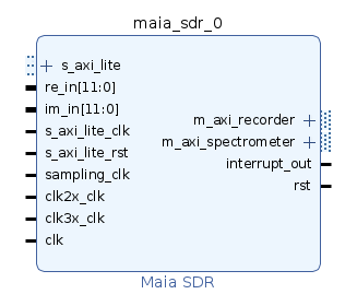
party designs. The top level of the design is an Amaranth
Elaboratable that gets synthesized to Verilog and packaged
as a Vivado IP core. As shown below, the IP core has re_in
and im_in ports for the IQ data of the ADC, an AXI4-Lite
subordinate interface to allow the ARM processor to control the core
through memory-mapped registers, AXI3 manager interfaces for the DMAs of
the spectrometer (waterfall) and IQ recorder, and ports for clocking and
reset.
The IP core is instantiated in the block design of a Vivado project that gets created and implemented using a TCL script. This is based on the build system used by Analog Devices for the default Pluto FPGA bitstream. In this respect, Maia SDR gives a good example of how Amaranth can be integrated in a typical flow using the Xilinx tools.
There are two classes of unit tests in maia-hdl. The first are Amaranth simulations. These use the Amaranth simulator, which is a Python simulator than can only simulate Amaranth designs. These tests give a simple but efficient and powerful way of testing Amaranth-only modules. The second are cocotb simulations. Cocotb is an open-source cosimulation testbench environment for verifying VHDL and Verilog designs using Python. Briefly speaking, it drives an HDL simulator using Python to control the inputs and check the outputs of the device under test. Cocotb has rich environment that includes Python classes that implement AXI devices. In maia-hdl, cocotb is used together with Icarus Verilog for the simulation of designs that involve Verilog modules (which happens in the cases in which we are instantiating from Amaranth a Xilinx primitive that is simulated with the Unisim library), and for those simulations in which the cocotb library is specially useful (such as for example, when using the cocotb AXI4-Lite Manager class to test our AXI4-Lite registers).
One of the driving features of Maia SDR is to optimize the FPGA resource utilization. This is important, because the Pluto Zynq-7010 FPGA is not so large, specially compared with other Xilinx FPGAs. To this end, Amaranth gives a good control about how the FPGA design will look like in terms of LUTs, registers, etc. The example with the counter has perhaps already shown that Amaranth is a low-level language, in the same sense that Verilog and VHDL are, and nothing comparable to HLS (where regular C code is translated to an FPGA design).
FFT
The main protagonist of the Maia SDR FPGA design is a custom pipelined FFT core that focuses on low resource utilization. In the Maia SDR Pluto firmware it is used as a radix-2² single-delay-feedback decimation-in-frequency 4096-point FFT with a Blackman-harris window. It can run at up to 62.5 Msps and uses only around 2.2 kLUTs, 1.4 kregisters, 9.5 BRAMs, and 6 DSPs. One of the tricks that allows to save a lot of DSPs is to use a single DSP for each complex multiplication, by performing the three required real products sequentially with a 187.5 MHz clock. A description of the design of the FFT core is out of the scope of this article, but I want to show a few features that showcase the strengths of Amaranth.
The first is the FFTControl module. The job of this
module is to generate the control signals for all the elements of the
FFT pipeline. In each clock cycle, it selects which operation each
butterfly should do, which twiddle factor should be used by each
multiplier, as well as the read and write addresses to use for the delay
lines that are implemented with BRAMs (these are used for the first
stages of the pipeline, which require large delay lines). As one can
imagine, these control outputs are greatly dependent on the
synchronization of all the elements. For example, if we introduce an
extra delay of one cycle in one of the elements, perhaps because we
register the data to satisfy timing constraints, all the elements
following this in the pipeline will need their control inputs to be
offset in time by one cycle.
It is really difficult to implement something like this in Verilog or VHDL. Changing these aspects of the synchronization of the design usually requires rethinking and rewriting parts of the control logic. In Amaranth, our modules are Python classes. We can have them “talk to each other” at synthesis time and agree on how the control should be set up, in such a way that the result will still work if we change the synchronization parameters.
For example, all the classes that are FFT pipeline elements implement
a delay Python @property that states what is
the input to output delay of the module measured in clock cycles. For
some simple modules this is always the same constant, but for a
single-delay-feedback butterfly it depends on the length of the delay
line of the butterfly, and for a twiddle factor multiplier it depends on
whether the multiplier is implemented with one or three DSPs. These are
choices that are done at synthesis time based on parameters that are
passed to the __init__() method of these modules.
The FFTControl module can ask at synthesis time to all
the elements that form the FFT pipeline what are their delays, and
figure out the reset values of some counters and the lengths of some
delay lines accordingly. This makes the control logic work correctly,
regardless what these delays are. For instance, the following method of
FFTControl computes the delay between the input of the FFT
and the input of each butterfly by summing up the delays of all the
preceding elements.
def delay_butterflies_input(self):
    """Gives the delay from the FFT input to the input of each of the
    butterflies"""
    return [
        self.delay_window
        + sum([butterfly.delay for butterfly in self.butterflies[:j]])
        + sum([twiddle.delay for twiddle in self.twiddles[:j]])
        for j in range(self.stages)
    ]
This is then used in the calculation of the length of some delay lines that supply the control signals to the butterflies. The code is slightly convoluted, but accounts for all possible cases. I don’t think it would be reasonable to do this kind of thing in Verilog or VHDL.
mux_bfly_delay = [
    [Signal(2 if isinstance(self.butterflies[j], R22SDF) else 1,
            name=f'mux_bfly{j}_delay{k}', reset_less=True)
     for k in range(0,
                    delay_butterflies_input[j]
                    - delay_twiddles_input[j-1]
                    + self.twiddles[j-1].twiddle_index_advance)]
     for j in range(1, self.stages)]
Another important aspect facilitated by Amaranth is the construction
of a model. We need a bit-exact model of our FFT core in order to be
able to test it in different situations and to validate simulations of
the Amaranth design against the model. Each of the modules that form the
pipeline has a model() method that uses NumPy to calculate
the output of that module given some inputs expressed as NumPy arrays.
Here is the model for a radix-2 decimation-in-frequency
single-delay-feedback butterfly. Perhaps it looks somewhat reasonable if
we remember that such a butterfly basically computes first
x[n] + x[n+v//2], for n = 0, 1, ..., v//2-1,
and then x[n] - x[n+v//2] for
n = 0, 1, ..., v//2-1.
[class R2SDF(Elaboratable):]
[...]
def model(self, re_in, im_in):
    v = self.model_vlen
    re_in, im_in = (np.array(x, 'int').reshape(-1, 2, v // 2)
                    for x in [re_in, im_in])
    re_out, im_out = [
        clamp_nbits(
            np.concatenate(
                (x[:, 0] + x[:, 1], x[:, 0] - x[:, 1]),
                axis=-1).ravel() >> self.trunc,
            self.w_out)
        for x in [re_in, im_in]]
    return re_out, im_out
The interesting thing is that, since each of the FFT pipeline modules
has its individual model, it is easy to verify the simulation of each
module against its model separately. The model of the FFT
module, which represents the whole FFT core, simply puts everything
together by calling the model() methods of each of the
elements in the pipeline in sequence. An important detail here is that
the arrays self._butterflies and
self._twiddles are the same ones that are used to
instantiate and connect together the pipeline modules, in terms of the
hardware design. By having these synergies between the model and the
hardware design, we reduce the chances of them getting out of sync due
to code changes.
[class FFT(Elaboratable):]
[...]
def model(self, re_in, im_in):
    v = self.model_vlen
    re = re_in
    im = im_in
    if self._window is not None:
        re, im = self._window.model(re, im)
    for j in range(self.nstages):
        re, im = self._butterflies[j].model(re, im)
        if j != self.nstages - 1:
            re, im = self._twiddles[j].model(re, im)
    return re, im
Instantiating Verilog modules and primitives
A question that often comes up is how to instantiate Verilog modules,
VHDL entities or FPGA primitives in an Amaranth design. Kate Temkin has
a short blog
post about it. In maia-hdl this is used in in several cases, such as
to implement clock domain crossing with the Xilinx FIFO18E1 primitive.
The most interesting example is however the Cmult3x module,
which implements complex multiplication with a single DSP48E1 that runs
at three clock cycles per input sample (some simple algebra shows that a
complex multiplication can be written with only three real
multiplications).
When designing modules with DSPs, I prefer to write HDL code that will make Vivado infer the DSPs I want. This is possible in simple cases, but in more complicated situations it is not possible to make Vivado understand exactly what we want, so we need to instantiate the DSP48 primitives by hand.
The drawback of having an Amaranth design that contains instances of Verilog modules, VHDL entities or primitives is that we can no longer simulate our design with the Amaranth simulator. If our instances have a Verilog model (such as is the case with Xilinx primitives via the Unisim library), we can still convert the Amaranth design to Verilog and use a Verilog simulator. This is done in maia-hdl using Icarus Verilog and cocotb. However, this can be somewhat inconvenient.
There is another possibility, which is to write different implementations of the same Amaranth module. One of them can be pure Amaranth code, which we will use for simulation, and another can use Verilog modules or primitives. The two implementations need to be functionally equivalent, but we can check this through testing.
The way to acomplish this is through Amaranth’s concept of platform.
The platform is a Python object that gets passed to the
elaborate() methods of the modules in the design. The
elaborate methods can then ask the platform for some objects that are
usually dependent on the FPGA family, such as flip-flop synchronizers.
This is a way of building designs that are more portable to different
families. The platform objects are also instrumental in the process of
building the bitstream completely within Amaranth, which is possible for
some FPGA families that have an open-source toolchain.
In the case of the maia-hdl Cmult3x we simply check
whether the platform we’ve been passed is an instance of
XilinxPlatform and depending on this we have the
elaborate() method either describe a pure Amaranth design
that models the DSP48 functionality that we need, or instantiate a
DSP48E1 primitive. Note that in the case of the pure Amaranth design we
do not model the full functionality of the DSP48. Only that which is
applicable to this use case.
[class Cmult3x(Elaboratable):]
[...]
def elaborate(self, platform):
    if isinstance(platform, XilinxPlatform):
        return self.elaborate_xilinx(platform)

    # Amaranth design. Vivado doesn't infer a single DSP48E1 as we want.
    [ ... here a pure amaranth design follows ... ]

def elaborate_xilinx(self, platform):
    # Design with an instantiated DSP48E1
    [...]
    m.submodules.dsp = dsp = Instance(
        'DSP48E1',
    [...]
Registers
Another aspect where the flexibility of Amaranth shines is in the
creation of register banks. In maia-hdl, the module
Register corresponds to a single 32-bit wide register and
the module Registers forms a register bank by putting
together several of these registers, each with their corresponding
address. The registers support a simple bus for reads and writes, and an
Axi4LiteRegisterBridge module is provided to translate
between AXI4-Lite and this bus, allowing the ARM CPU to access the
registers.
Registers and register banks are created with Python code that
describes the fields of the registers. The basic ingredient is the
Field named tuple:
Field = collections.namedtuple('RegisterField',
                               ['name', 'access', 'width', 'reset'])
We describe a register by giving it a name, an access mode (which can be read-only, write-only, read-write, or some other more specialized modes that we will describe below), a width, and a reset or default value.
The best way to understand how to work with these registers is to see how they are used in the Maia SDR top-level design.
self.control_registers = Registers(
    'control',
    {
        0b00: Register(
            'product_id', [
                Field('product_id', Access.R, 32, 0x6169616d)
            ]),
        0b01: Register('version', [
            Field('bugfix', Access.R, 8,
                  int(_version.split('.')[2])),
            Field('minor', Access.R, 8,
                  int(_version.split('.')[1])),
            Field('major', Access.R, 8,
                  int(_version.split('.')[0])),
            Field('platform', Access.R, 8, 0),
        ]),
        0b10: Register('control', [
            Field('sdr_reset', Access.RW, 1, 1),
        ]),
        0b11: Register('interrupts', [
            Field('spectrometer', Access.Rsticky, 1, 0),
            Field('recorder', Access.Rsticky, 1, 0),
        ], interrupt=True),
    },
    2)
self.recorder_registers = Registers(
    'recorder',
    {
        0b0: Register('recorder_control', [
            Field('start', Access.Wpulse, 1, 0),
            Field('stop', Access.Wpulse, 1, 0),
            Field('mode_8bit', Access.RW, 1, 0),
            Field('dropped_samples', Access.R, 1, 0),
        ]),
        0b1: Register('recorder_next_address', [
            Field('next_address', Access.R, 32, 0),
        ]),
    },
    1)
Here we show two register banks: one for the control of the IP core and another for the control of the IQ recorder. There is a similar third register bank for the control of the spectrometer (waterfall).
The parameters of the Registers constructor are a name,
a dictionary that contains the registers in the bank (the keys of the
dictionary are the addresses, and the values are the
Register objects), and the width of the address bus. Note
that these addresses correspond to the addressing of the native register
bus. When we convert to AXI4-Lite, the addresses get shifted by two bits
to the left because each register is 4 bytes wide.
The parameters of the Register constructor are a name
and a list of Field‘s describing the fields of the
register. Fields are allocated into the 32-bit register according to
their order in the list, starting by the LSB. For instance, in the
interrupts register, the spectrometer field
occupies the LSB and the recorder field occupies the next
bit.
If we look at the control registers, we can see that the
registers for product_id and version have
access type R, which means read-only. These registers are
never wired in the design to other signals that would override their
default values, so they are in fact constants that the CPU can read to
check that the IP core is present and find its version number.
Next we have a control register, which has an
sdr_reset field. This is wired internally to a bunch of
reset signals in the IP core. It has a default value of 1, which means
that most of the IP core starts in reset. The CPU can write a 0 to this
field to take the IP core out of reset before using it. Accessing this
sdr_reset field within the design is very simple, because
the Registers and Register implement
__getitem__(), allowing us to access them as if they were
dictionaries. This example shows how it works. Here we are connecting
the field sdr_reset to the reset input of something called
rxiq_cdc (which implements clock domain crossing between
the ADC sampling clock and the internal clock used in the IP core).
m.d.comb += rxiq_cdc.reset.eq(
    self.control_registers['control']['sdr_reset'])
If we look at the interrupts register, we can see an
example of the Rsticky access mode. This means read-only
sticky. A field of this type will be set to 1 when its input (which is
wired internally in the IP core) has the value 1. It will keep the value
1 even if the input goes back to 0. The field is cleared and set to 0
when it is read. The intended use for this access mode is interrupts. A
module can pulse the input of the field to notify an interrupt, and the
field will hold a 1 until the CPU reads the register, clearing the
interrupts. The interrupts register even has an
interrupt=True option that provides an interrupt output
that can be connected directly to the F2P interrupt port of the Zynq.
This interrupt output will be high whenever any Rsticky
field in the register is non-zero.
Finally, the recorder_control field gives some examples
of the Wpulse access type. This is a write-only field with
pulsed output. Writing a 1 to this field causes a one-cycle pulse at its
output. This is ideal for controlling modules that require a pulse to
indicate some event or command. For example, this is the case with the
start and stop commands of the IQ recorder.
The Amaranth code that makes all of this work is not so complicated.
You can take a look at the register.py file in maia-hdl to
see for yourself.
Another interesting feature of this register system is that it can write an SVD file describing the register map. CMSIS-SVD is an XML format that is often used to describe the register maps of microcontrollers and SoCs. Maia SDR uses svd2rust to generate a nice Rust API for register access.
The Registers and Register classes have
svd() methods that generate the SVD XML using Python’s
xml.etree.ElementTree. This is relatively simple, because
the classes already have all the information about these registers. It
is, after all, the same information that they use to describe the
hardware implementation of the registers. This is another example of how
by using synergies between the code that describes the hardware design
and code that does something related to that hardware design (in this
case, writing SVD), we make it harder for changes in the code base to
cause inconsistencies.
Conclusions
In this article we have gone from a “hello world” type counter in Amaranth to some rather intricate code from the inner workings of an FFT core. My intention with giving these code examples is not to expect the reader to understand all the code, but rather to give a feeling for how using Amaranth in complex projects can look like. Perhaps by now I have managed to convince you that Amaranth is a powerful and flexible alternative to HDLs such as Verilog and VHDL, or at least to get you interested in learning more about Amaranth and the world of open-source FPGA and silicon design.
Federal Communications Commission Technological Advisory Council resumes!
Want someone on your side at the FCC? We have good news. The FCC TAC is going to resume work. The previous term ended in December 2022 with an in-person meeting in Washington, DC. ORI was a member of the AI/ML Working Group and served as a co-chair of the “Safe Uses of AI/ML” sub-working group. The next term will be for two years. The appointment will require another round of nominations and vetting. An invitation to ORI has been made. ORI will speak up for open source digital radio work and the amateur radio services. Thank you to everyone that made the 2022 FCC TAC term productive and beneficial. Join the #ai channel on ORI Slack to get more involved. Not part of Slack? Visit https://openresearch.institute/getting-started to Get Started.
HDL Coder for Software Defined Radio Class May 2023
Sign-ups are live at https://us.commitchange.com/ca/san-diego/open-research-institute/campaigns/hdl-coder-for-software-defined-radio
Advanced training for Digital Communications, Software Defined Radio, and FPGAs will be held 1-5 May 2023. Do you know someone that can benefit from customized and focused training? Please forward this email to them. Designed to benefit open source digital radio, this course also benefits the amateur radio services.
Presented by ORI and taught by Mathworks, this class will cover the following topics.
COURSE OUTLINE
Day 1 – Generating HDL Code from Simulink & DSP for FPGAs
Preparing Simulink Models for HDL Code Generation (1.0 hrs)
Prepare a Simulink model for HDL code generation. Generate HDL code and testbench for simple models requiring no optimization.
- Preparing Simulink models for HDL code generation
- Generating HDL code
- Generating a test bench
- Verifying generated HDL code with an HDL simulator
Fixed-Point Precision Control (2.0 hrs)
Establish correspondence between generated HDL code and specific Simulink blocks in the model. Use Fixed-Point Tool to finalize fixed point architecture of the model.
- Fixed-point scaling and inheritance
- Fixed-Point Designer workflow
- Fixed-Point Tool
- Fundamental adders and multiplier arrays
- Division and square root arrays
- Wordlength issues and Fixed-point arithmetic
- Saturate and wraparound.
- Overflow and underflow
Optimizing Generated HDL Code (4 hrs)
Use pipelines to meet design timing requirements. Use specific hardware implementations and share resources for area optimization.
- Generating HDL code with the HDL Workflow Advisor
- Meeting timing requirements via pipelining
- Choosing specific hardware implementations for compatible Simulink blocks
- Sharing FPGA/ASIC resources in subsystems
- Verifying that the optimized HDL code is bit-true cycle-accurate
- Mapping Simulink blocks to dedicated hardware resources on FPGA
Day 2 – DSP for FPGAs
Signal Flow Graph (SFG) Techniques (SFG) Techniques and high-speed FIR design (2.0 hrs)
Review the representation of DSP algorithms using signal flow graph. Use the Cut Set method to improve timing performance. Implement parallel and serial FIR filters.
- DSP/Digital Filter Signal Flow Graphs
- Latency, delays and “anti-delays”!
- Re-timing: Cut-set and delay scaling
- The transpose FIR
- Pipelining and multichannel architectures
- SFG topologies for FPGAs
- FIR filter structures for FPGAs
Multirate Signal Processing for FPGAs (4.0 hrs)
Develop polyphase structure for efficient implementation of multirate filters. Use CIC filter for interpolation and decimation.
- Upsampling and interpolation filters
- Downsampling and decimation filters
- Efficient arithmetic for FIR implementation
- Integrators and differentiators
- Half-band, moving average and comb filters
- Cascade Integrator Comb (CIC) Filters (Hogenauer)
- Efficient arithmetic for IIR Filtering
CORDIC Techniques AND channelizers (2.0 hrs)
Introduce CORDIC algorithm for calculation of various trigonometric functions.
- CORDIC rotation mode and vector mode
- Compute cosine and sine function
- Compute vector magnitude and angle
- Architecture for FPGA implementation
- Channelizer
Day 3 – Programming Xilinx Zynq SoCs with MATLAB and Simulink & Software-Defined Radio with Zynq using Simulink
IP Core Generation and Deployment (2.0 hrs)
Use HDL Workflow Advisor to configure a Simulink model, generate and build both HDL and C code, and deploy to Zynq platform.
- Configuring a subsystem for programmable logic
- Configuring the target interface and peripherals
- Generating the IP core and integrating with SDK
- Building and deploying the FPGA bitstream
- Generating and deploying a software interface model
- Tuning parameters with External Mode
Model Communications System using Simulink (1.5 hrs)
Model and simulate RF signal chain and communications algorithms.
- Overview of software-defined radio concepts and workflows
- Model and understand AD9361 RF Agile Transceiver using Simulink
- Simulate a communications system that includes a transmitter, AD9361 Transceiver, channel and Receiver (RF test environment)
Implement Radio I/O with ADI RF SOM and Simulink (1.5 hrs)
Verify the operation of baseband transceiver algorithm using real data streamed from the AD9361 into MATLAB and Simulink.
- Overview of System object and hardware platform
- Set up ADI RF SOM as RF front-end for over-the-air signal capture or transmission
- Perform baseband processing in MATLAB and Simulink on captured receive signal
- Configure AD9361 registers and filters via System object
- Verify algorithm performance for real data versus simulated data
Prototype Deployment with Real-Time Data via HW/SW Co-Design (2.0 hrs)
Generate HDL and C code targeting the programmable logic (PL) and processing system (PS) on the Zynq SoC to implement TX/RX.
- Overview of Zynq HW/SW co-design workflow
- Implement Transmitter and Receiver on PL/PS using HW/SW co-design workflow
- Configure software interface model
- Download generated code to the ARM processor and tune system parameters in real-time operation via Simulink
- Deploy a stand-alone system
FPGA Workshop Cruise with ORI?
Want to learn more about open source FPGA development from experts in the field? Ready to capitalize on the HDL Coder for Software Defined Radio Class happening in May 2023? Want to get away? How about something that can give you both? We are looking at organizing an FPGA Workshop Adventure Cruise. Be part of the planning and write fpga@openresearch.institute
Are you interested in supporting work at ORI?
Consider being part of the board. We’d like to expand from 5 to 7 members in order to better serve our projects and community.
We’ve got lots going on with Opulent Voice, Haifuraiya, AmbaSat Respin, and regulatory work.
Thank you from everyone at ORI for your continued support and interest!
Want to be a part of the fun? Get in touch at ori@openresearch.institute